Decomposing funnel metrics
Table of contents
Funnel metrics as products
I talked about metric decomposition in a previous article, and how it can be used to explain why metrics change values over time. That article explained how to decompose a sum, as well as a ratio. In this article, I’ll explain how to decompose a product.
revenue = impressions * click_rate * conversion_rate * spend
The decomposition in this article isn’t limited to funnels. It can be applied to any metric that is expressed as a product of factors. For instance, at Carbonfact, we decompose the carbon footprint of a clothing line as so:
footprint = products * kg_per_product * footprint_per_kg
This allows us to understand whether a clothing line’s total footprint has increased – or decreased – because of an increase in the number of products, an increase in the weight of each product, or an increase in the footprint intensity of each product.
The intuition
Let’s take a typical revenue funnel as an example. People come to a website, which are counted as impressions. They are presented with a CTA, which may or not result into a click. Each user may then subscribe to a service, or not. Each user will then spend some money through their subscription, which is often defined as their LTV. This funnel has 4 steps:
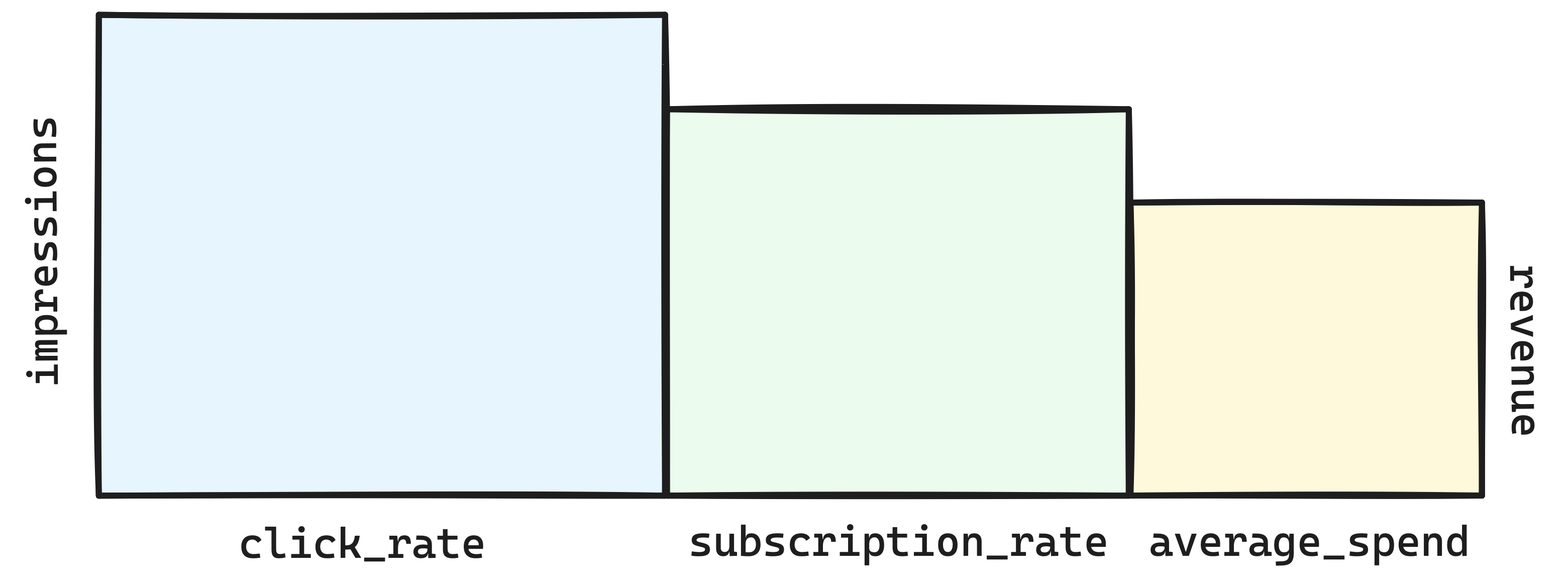
The revenue of this website can be expressed as a product of four factors:
revenue = impressions * click_rate * subscription_rate * average_spend
Let’s say the revenue changes between two time periods. We want to understand why. The overall change can be attributed to a change in any of the factors. For example, the revenue may have increased because of an increase in the number of impressions, or because of an increase in the subscription rate. Decomposing the change would allow us attribute part of the change to each of the funnel’s steps.
Let’s focus on the amount of clicks. The number of clicks can change between two periods for two reasons:
- The number of impressions changed.
- The click rate evolved.
Let’s say both of these factors increased. This is illustrated in the following figure:

The increase in number of clicks can be decomposed as the sum of two terms:
- The increase in number of impressions, multiplied by the click rate:
$$ (I’ - I) \times C $$
- The increase in click rate, multiplied by the new number of impressions:
$$ I’ \times (C’ - C) $$
The first term would be attributed to impressions evolutions, whilst the second would be attributed to the click rate change. Note that this is a purely geometric intepretation. An alternative slicing is shown in the following figure:

This is the same story as in the previous article. The take-away is that there are different ways to decompose a metric, and that all of them are valid. Each one gives slightly different results, but they all yield figures with the same order of magnitude.
In both cases, the decomposition provides the contribution of each factor to the evolution of the amount of clicks. What we want is the contribution to the evolution of the overall revenue. This can be obtained by multiplying each contribution by the other factors, namely the subscription rate $S$ and the average spend $A$. All in all, the decomposition of the revenue evolution is:
$$ \textcolor{royalblue}{(I’ - I) \times C \times S \times A} + \textcolor{indianred}{I’ \times (C’ - C) \times S \times A} $$
One may ask why we would use the previous subscription rate and average spend, rather than the new values. The easy answer is that this wouldn’t add up mathematically. The more intuitive answer is that the contribution of a factor’s evolution should comprise the change of the attribute itself, as well as the change of the factors that precede it. Indeed, if the click rate increases, then its contribution should be compounded by the fact that there are more impressions.
The math
We’ve established a funnel metric $m$ can be expressed a product of $k$ factors $f_i$:
$$ m = \prod_{i=1}^k f_i $$
We’re interested in explaining the evolution of the metric over time. The metric can be indexed with a timestamp $t$:
$$ m_t = \prod_{i=1}^k f_{i,t} $$
The metric’s evolution between two timestamps $t$ and $t’$ – which doesn’t necessarily have to be $t+1$ – can be expressed as:
$$ m_{t’} - m_t = \prod_{i=1}^k f_{i,t’} - \prod_{i=1}^k f_{i,t} $$
This difference is a single number. We want to decompose it into a sum of factors. That is, we want to measure the contribution of each factor to the metric’s evolution. Each factor’s contribution should be proportional to said factor’s evolution between $t$ and $t’$.
Our goal is to understand the impact of this change on the overall metric change. Therefore, we want a factor’s contribution to be expressed as a function of $f_{i,t’} - f_{i,t}$. I haven’t yet derived the formula here, but the final result is:
$$ m_{t’} - m_t = \sum_{i=1}^k \left( \textcolor{royalblue}{\prod_{j=1}^{i-1} f_{j,t’}} \times \textcolor{purple}{(f_{i,t’} - f_{i,t})} \times \textcolor{indianred}{\prod_{j=i+1}^k f_{j,t}} \right) $$
This is mathematical equivalent to the geometric explanation from above. The purple term is the factor’s evolution. The blue term is the product of the factors that precede the factor of interest, evaluated at the new timestamp. The red term is the product of the factors that follow the factor of interest, evaluated at the old timestamp.
Note that an alternative decomposition is:
$$ m_{t’} - m_t = \sum_{i=1}^k \left( \textcolor{royalblue}{\prod_{j=1}^{i-1} f_{j,t}} \times \textcolor{purple}{(f_{i,t’} - f_{i,t})} \times \textcolor{indianred}{\prod_{j=i+1}^k f_{j,t’}} \right) $$
where we intervert the timestamps in the blue and red terms. This is the same as the previous decomposition, but with the timestamps swapped. There is no better formula. Both are valid, and simply differ in interpretation. The first decomposition compounds the change with the factors that precede the factor of interest, whilst the second compounds the change with the factors that follow.
Python code
Here’s a toy dataset to illustrate:
See code
import pandas as pd

df = pd.DataFrame({
    'date': ['2018-01-01', '2018-01-01', '2018-01-01', '2019-01-01', '2019-01-01', '2019-01-01', '2018-02-01', '2018-02-01', '2018-02-01', '2019-02-01', '2019-02-01', '2019-02-01'],
    'group': ['A', 'B', 'C', 'A', 'B', 'C', 'A', 'B', 'C', 'A', 'B', 'C'],
    'impressions': [1000, 2000, 2500, 1000, 2150, 2000, 50, 2000, 2500, 2500, 2150, 2000],
    'clicks': [150, 150, 250, 120, 200, 400, 20, 300, 250, 1000, 323, 320],
    'conversions': [120, 150, 125, 100, 145, 166, 10, 150, 125, 500, 145, 166],
    'revenue': ['$8,600', '$9,400', '$10,750', '$9,055', '$8,739', '$10,147', '$500', '$11,400', '$8,750', '$50,000', '$10,739', '$12,147'],
})
df['date'] = pd.to_datetime(df['date'])
df['revenue'] = df['revenue'].str.replace('$', '', regex=False).str.replace(',', '', regex=False).astype(float)
df
| date | group | impressions | clicks | conversions | revenue |
|---|---|---|---|---|---|
| 2018-01-01 | A | 1000 | 150 | 120 | 8600 |
| 2018-01-01 | B | 2000 | 150 | 150 | 9400 |
| 2018-01-01 | C | 2500 | 250 | 125 | 10750 |
| 2019-01-01 | A | 1000 | 120 | 100 | 9055 |
| 2019-01-01 | B | 2150 | 200 | 145 | 8739 |
| 2019-01-01 | C | 2000 | 400 | 166 | 10147 |
| 2018-02-01 | A | 50 | 20 | 10 | 500 |
| 2018-02-01 | B | 2000 | 300 | 150 | 11400 |
| 2018-02-01 | C | 2500 | 250 | 125 | 8750 |
| 2019-02-01 | A | 2500 | 1000 | 500 | 50000 |
| 2019-02-01 | B | 2150 | 323 | 145 | 10739 |
| 2019-02-01 | C | 2000 | 320 | 166 | 12147 |
The overall change in revenue between 2018 and 2019 is:
(
    df.assign(year=df.date.dt.year)
    .groupby('year')
    .agg({'revenue': 'sum'})
    .diff()
    .dropna()
)
51427
That’s the total amount we want to explain. The first step is to define the funnel’s factors:
funnel = ['impressions', 'clicks', 'conversions', 'revenue']
This list can then be used to create additional ratio columns:
ratio_names = [
    f'{num}_over_{den}' if den else num
    for den, num in [(None, funnel[0]), *zip(funnel, funnel[1:])]
]
ratio_names
[
    'impressions',
    'clicks_over_impressions',
    'conversions_over_clicks',
    'revenue_over_conversions'
]
decomp = df.copy()
for name, den, num in zip(ratio_names, funnel, funnel[1:]):
    decomp[name] = df[num] / df[den]
decomp
| date | group | impressions | clicks_over_impressions | conversions_over_clicks | revenue_over_conversions |
|---|---|---|---|---|---|
| 2018-01-01 | A | 1000 | 15% | 80% | $72 |
| 2018-01-01 | B | 2000 | 7.5% | 100% | $63 |
| 2018-01-01 | C | 2500 | 10% | 50% | $86 |
| 2019-01-01 | A | 1000 | 12% | 83% | $57 |
| 2019-01-01 | B | 2150 | 9% | 72.5% | $60 |
| 2019-01-01 | C | 2000 | 20% | 41.5% | $61 |
| 2018-02-01 | A | 50 | 40% | 50% | $50 |
| 2018-02-01 | B | 2000 | 15% | 50% | $76 |
| 2018-02-01 | C | 2500 | 10% | 50% | $70 |
| 2019-02-01 | A | 2500 | 40% | 50% | $100 |
| 2019-02-01 | B | 2150 | 15% | 45% | $74 |
| 2019-02-01 | C | 2000 | 16% | 52% | 73 |
I’ve formatted the columns for readability. In practice, you might have these columns directly available, and won’t need to create them. The next step is to define the dimensions along which to decompose the evolution:
dimensions = ['month', 'group']
This then allows us to add additional columns that allow comparing the current ratios to the previous ones. This can be done with pandas’ shift method:
decomp['month'] = decomp.date.dt.month
for name in ratio_names:
    decomp[f'{name}_lag'] = decomp.groupby(dimensions)[name].shift(1)
We can finally apply the decomposition formula one factor at a time:
for i, _ in enumerate(ratio_names):

    before = ratio_names[:i]
    current = f'({ratio_names[i]} - {ratio_names[i]}_lag)'
    after = [f'{x}_lag' for x in ratio_names[i+1:]]
    formula = ' * '.join(filter(None, [*before, current, *after]))

    decomp[f'{ratio_names[i]}_contribution'] = decomp.eval(formula)

decomp
| date | group | impressions_contribution | clicks_over_impressions_contribution | conversions_over_clicks_contribution | revenue_over_conversions_contribution |
|---|---|---|---|---|---|
| 2019-01-01 | A | $0 | -$1720 | $286.667 | $1888.33 |
| 2019-01-01 | B | $705 | $2428.33 | -$3446.67 | -$347.667 |
| 2019-01-01 | C | -$2150 | $8600 | -$2924 | -$4129 |
| 2019-02-01 | A | $24500 | $0 | $0 | $25000 |
| 2019-02-01 | B | $855 | $19 | -$1254 | -$281 |
| 2019-02-01 | C | -$1750 | $4200 | $420 | $527 |
We observe that the highest contributor to the revenue growth of Februrary 2019 is the increase in average spend. This makes sense, because the average spend increased by $25,000. Meanwhile, the number of conversions slightly decreased for group B in both January and February, each time resulting in a negative contribution to revenue. I think it’s very powerful to be able to attribute a loss of revenue to a specific factor this way.
Note that the contribution columns can be summed up to verify the decomposition is valid:
contribution_columns = [x for x in decomp.columns if x.endswith('_contribution')]
(
    decomp
    .assign(year=x.date.dt.year)
    .groupby('year')[contribution_columns].sum().sum(axis=1)
)
51427
This is a good sanity check if you’re going to implement this yourself.
Towards a general solution
Alas I don’t have time to dive more into this. I’ve just had a baby and don’t have the leasure to write as I used to. I wanted to put this on paper while the topic was hot in my mind. I will come back to it later, and hopefully derive a more general solution that can be applied to any metric formula. Indeed, the previous article and this one cover sums, ratios, and products. I suspect there is a general decomposition framework that can be applied to any formula.