Bayesian linear regression for practitioners
Table of contents
Motivation
Suppose you have an infinite stream of feature vectors $x_i$ and targets $y_i$. In this case, $i$ denotes the order in which the data arrives. If you’re doing supervised learning, then your goal is to estimate $y_i$ before it is revealed to you. In order to do so, you have a model which is composed of parameters denoted $\theta_i$. For instance, $\theta_i$ represents the feature weights when using linear regression. After a while, $y_i$ will be revealed, which will allow you to update $\theta_i$ and thus obtain $\theta_{i+1}$. To perform the update, you may apply whichever learning rule you wish – for instance most people use some flavor of stochastic gradient descent. The process I just described is called online supervised machine learning. The difference between online machine learning and the more traditional batch machine learning is that an online model is dynamic and learns on the fly. Online learning solves a lot of pain points in real-world environments, mostly because it doesn’t require retraining models from scratch every time new data arrives.
Most of the popular online machine learning models are built around some form of stochastic gradient descent. Moreover, they are typically used to make point predictions via maximum likelihood estimation. A different – and generally more desirable – approach is to estimate $y_i$ by using a distribution. In other words, instead of predicting the most likely output, we would rather like to get an idea of the spread of values that $y_i$ might take. Having a distribution instead of a single value gives an idea of the uncertainty of the model, which is obviously a nice thing to have. Such is one of the many benefits of using Bayesian inference.
Bayesian inference with colors
I’ve stumbled on many blogs, posts, textbooks, slides, that discussed Bayesian inference. In my opinion, it’s a hard topic, and it has many rabbit holes that go on for ever. Chapter 3 of Christopher Bishop’s classical book is a very good reference, but it leaves me unsatisfied with regards to practical aspects – the book is not available for free, but these slides contain all the material from chapter 3 on Bayesian linear regression. This is mostly because I am too lazy to take the time required to understand everything written in Bishop’s book. Here’s a bunch of blog posts that helped me get a clearer understanding:
- Sequential Bayesian Learning - Linear Regression by dtransposed
- Bayesian/Streaming Algorithms by Vincent Warmerdam
- Bayesian Linear Regression Tutorial by zjost
- Sequential Bayesian linear regression by Daniel Daza
In this post I would like to present a (my) pragmatic view of Bayesian inference, focused on online machine learning and practical aspects. Before getting into the code, I would like to give a generic overview of the topic. However, if you’re in a hurry and want to dig into the code straight away, feel free to move on forward. I’ve purposefully chosen a mathematical notation that is particularly well suited to online machine learning. I’ve taken a bit of freedom with regards to the notation; if you’re part of the mathematical inquisition then take a chill pill. Note that there will probably be a fair bit of overlap with the blog posts I listed above, but I don’t think that matters too much.
This is the distribution we want to obtain. It’s the Holy Grail for many practitioners who want to take into account predictive uncertainty. Later on we’ll see how the predictive distribution is obtained by assembling the rest of the blocks.
The thing to understand is that the likelihood is usually imposed by the problem you’re dealing with. In textbooks, the likelihood is often chosen to be a Gaussian or a binomial, mostly because these distributions occur naturally in textbook problems. However, the likelihood can be any parametric distribution. The key idea is that the likelihood is something defined by the problem at hand, and usually isn’t something you have to much freedom with.
Choosing a prior is important, because for our case it can add regularization to our model. The trick is that if we choose a prior distribution that is so-called conjugate for the likelihood, then we get access to analytical formulas for updating the model parameters. If, however, the prior and the likelihood are not compatible with each other, then we have to resort to using approximate methods such as MCMC and variational inference. As cool and trendy as they may be, these tools are mostly designed for situations where all the data is available at once. In other words they are not applicable in a streaming context, whereas analytical formulas are.
As you might have guessed or already know, the posterior distribution is obtained by combining the likelihood of $(x_{i}, y_{i})$ and the prior distribution of the current model parameters $\theta_{i}$. As a mnemonic, red $+$ blue $=$ purple .
Now that we have all our blocks, we need to put them together. It’s quite straightforward once you understand how the blocks are related. You start off with the likelihood, which is a probability distribution you have to choose. For example if you’re looking to predict counts then you would use a Poisson distribution. I’m refraining from giving a more detailed example simply because we will be going over one later on. What matters for the while is to develop an intuition, and for that I want to keep the notation as general as possible. Once you have settled on a likelihood, you need to choose a prior distribution for the model parameters. Because our focus is on online learning, we want to have access to quick analytical formulas, and not MCMC voodoo. In order to so, we need to pick a prior distribution which is conjugate to the likelihood. Note that most distributions have at least one other distribution which is conjugate to them, as detailed here. Now that you have decided which likelihood to use and what prior to associate with it, you may derive the posterior distribution of the model parameters. This operation is the cornerstone of Bayesian inference, and is done via Bayes’ rule:
$$\begin{equation} \textcolor{mediumpurple}{p(\theta_{i+1} | \theta_i, x_i, y_i)} = \frac{\textcolor{indianred}{p(y_i | x_i, \theta_i)} \textcolor{royalblue}{p(\theta_i)}}{p(x_i, y_i)} \end{equation}$$
Now you may be wondering what $p(x_i, y_i)$ is. It turns out it is the distribution of the data, and is something that we don’t know! Indeed, if we knew the generating process of the data, then we wouldn’t really have to be doing machine learning in the first place, right? There are however analytical formulas that use the rest of the information at our disposal – namely the prior and the likelihood – but they require the likelihood and the prior to be conjugate to each other. These formulas involve a sequence of mathematical steps which we will omit. All you have to know is that if the prior and the likelihood are conjugate to each other, then an analytical formula for computing the posterior is available, which allows us to perform online learning. To keep things general, we will simply write down:
$$\begin{equation} \textcolor{mediumpurple}{p(\theta_{i+1} | \theta_i, x_i, y_i)} \propto \textcolor{indianred}{p(y_i | x_i, \theta_i)} \textcolor{royalblue}{p(\theta_i)} \end{equation}$$
The previous statement simply expresses the fact that the posterior distribution of the model parameters is proportional to the product of the likelihood and the prior distribution. In other words, in can be obtained using an analytical formula that is specific to the chosen likelihood and prior distribution. If we’re being pragmatic, then what we’re really interested in is to obtain the predictive distribution, which is obtained by marginalizing over the model parameters $\theta_i$:
$$\begin{equation} \textcolor{forestgreen}{p(y_i | x_i)} = \int \textcolor{indianred}{p(y_i | \textbf{w}, x_i)} \textcolor{royalblue}{p(\textbf{w})} d\textbf{w} \end{equation}$$
Again, this isn’t analytically tractable, except if the likelihood and the prior are conjugate to each other. The equation does make sense though, because essentially we’re computing a weighted average of the potential $y_i$ values for each possible model parameter $\textbf{w}$.
$$\begin{equation} \textcolor{forestgreen}{p(y_i | x_i)} \propto \textcolor{indianred}{p(y_i | x_i, \theta_i)} \textcolor{royalblue}{p(\theta_i)} \end{equation}$$
Basically, the thing to remember is that the predictive distribution can be obtained by mixing the likelihood and the current distribution of the weights.
Online belief updating
The important result of the previous section is that we can get update the distribution of the parameters when a new pair $(x_i, y_i)$ arrives:
$$\begin{equation} \textcolor{mediumpurple}{p(\theta_{i+1} | \theta_i, x_i, y_i)} \propto \textcolor{indianred}{p(x_i, y_i | \theta_i)} \textcolor{royalblue}{p(\theta_i)} \end{equation}$$
Before any data comes in, the model parameters follow the initial distribution we picked, which is $p(\theta_0)$. At this point, if we’re asked to predict $y_0$, then it’s predictive distribution would be obtained as so:
$$\begin{equation} \textcolor{forestgreen}{p(y_0 | x_0)} \propto \textcolor{indianred}{p(y_0 | x_0, \theta_0)} \textcolor{royalblue}{p(\theta_0)} \end{equation}$$
Next, once the first observation $(x_0, y_0)$ arrives, we can update the distribution of the parameters:
$$\begin{equation} \textcolor{mediumpurple}{p(\theta_1 | \theta_0, x_0, y_0)} \propto \textcolor{indianred}{p(x_0, y_0 | \theta_0)} \textcolor{royalblue}{p(\theta_0)} \end{equation}$$
The predictive distribution, given a set of features $x_1$, is thus:
$$\begin{equation} \textcolor{forestgreen}{p(y_1 | x_1)} \propto \textcolor{indianred}{p(y_1 | x_1, \theta_1)} \underbrace{\textcolor{mediumpurple}{p(\theta_1 | \theta_0, x_0, y_0)}}_{\textcolor{royalblue}{p(\theta_1)}} \end{equation}$$
The previous equations expresses the fact that the prior of the weights for the current iteration is the posterior of the weights at the previous iteration. Once the second pair $(x_1, y_1)$ is available, the distribution of the model parameters is updated in the same way as before:
$$\begin{equation} \textcolor{mediumpurple}{p(\theta_2 | \theta_1, x_1, y_1)} \propto \textcolor{indianred}{p(y_1 | x_1, \theta_1)} \underbrace{\textcolor{indianred}{p(y_0 | x_0, \theta_0)} \textcolor{royalblue}{p(\theta_0)}}_{\textcolor{royalblue}{p(\theta_1)}} \end{equation}$$
When the pair $(x_2, y_2)$ arrives, the distribution of the weights will be obtained as so:
$$\begin{equation} \textcolor{mediumpurple}{p(\theta_3 | \theta_2, x_2, y_2)} \propto \textcolor{indianred}{p(y_2 | x_2, \theta_2)} \underbrace{\textcolor{indianred}{p(y_1 | x_1, \theta_1)} \underbrace{\textcolor{indianred}{p(y_0 | x_0, \theta_0)} \textcolor{royalblue}{p(\theta_0)}}_{\textcolor{royalblue}{p(\theta_1)}} }_{\textcolor{royalblue}{p(\theta_2)}} \end{equation}$$
Hopefully, by now you’ve understood that there is recursive relationship that links each iteration: the posterior distribution at step $i$ becomes the prior distribution at step $i+1$. This simple fact is the reason why analytical Bayesian inference can naturally be used as an online machine learning algorithm. Indeed, we only need to store the current distribution of the weights to make everything work. When I started to understand this for the first time, I found it slightly magical.
On a sidenote, I want to mention that this presentation of Bayesian inference is very much “old school”. Most people who do Bayesian inference use MCMC and variational inference techniques. These tools are really cool, and I highly recommend checking out libraries such as Stan, PyMC3 – (and PyMC4 which will be it’s successor), Edward, and Pyro. The issue with these tools is that they require having all the training data available in memory, and thus are not able to learn in an online manner. There do however seem to be some variants that work online, such as sequential Monte Carlo and stochastic variational inference. In my experience these algorithms work well for mini-batches, but not necessarily in a pure online setting where the observations are processed one-by-one. I will probably be discussing these methods in a future blog post.
The case of linear regression
Up until now we didn’t give any useful example. We will now see how to perform linear regression by using Bayesian inference. In a linear regression, the model parameters $\theta_i$ are just weights $w_i$ that are linearly applied to a set of features $x_i$:
$$\begin{equation} y_i = w_i x_i^\intercal + \epsilon_i \end{equation}$$
Each prediction is the scalar product between $p$ features $x_i$ and $p$ weights $w_i$. The trick here is that we’re going to assume that the noise $\epsilon_i$ follows a given distribution. In particular, we will be boring and use the Gaussian ansatz, which implies that the likelihood function is a Gaussian distribution:
$$\begin{equation} \color{indianred} p(y_i | x_i, w_i) = \mathcal{N}(w_i x_i^\intercal, \beta^{-1}) \end{equation}$$
Christopher Bishop calls $\beta$ the “noise precision parameter”. In statistics, the precision is inversely related to the noise variance as so: $\beta = \frac{1}{\sigma^2}$. Basically, it translates our belief on how noisy the target distribution is. Both concepts coexist mostly because statisticians can’t agree on a common Bible. There are ways to tune this parameter automatically from the data. However, for the purpose of simplicity, in this blog post we will “treat it as a known constant” – I’m quoting Christopher Bishop. In any case, the appropriate prior distribution for the above likelihood function is the multivariate Gaussian distribution:
$$\begin{equation} \color{royalblue} p(w_0) = \mathcal{N}(m_0, S_0) \end{equation}$$
$m_0$ is the mean of the distribution while $S_0$ is it’s covariance matrix. Initially, their initial values will be:
$$\begin{equation} m_0 = (0, \dots , 0) \end{equation}$$
$$\begin{equation} S_0 = \begin{pmatrix} \alpha^{-1} & \dots & \dots \\ \dots & \alpha^{-1} & \dots \\ \dots & \dots & \alpha^{-1} \end{pmatrix} \end{equation}$$
We can now determine the posterior distribution of the weights:
$$\begin{equation} \color{mediumpurple} p(w_{i+1} | w_i, x_i, y_i) = \mathcal{N}(m_{i+1}, S_{i+1}) \end{equation}$$
$$\begin{equation} S_{i+1} = (S_i^{-1} + \beta x_i^\intercal x_i)^{-1} \end{equation}$$
$$\begin{equation} m_{i+1} = S_{i+1}(S_i^{-1} m_i + \beta x_i y_i) \end{equation}$$
Note that $x_i^\intercal x_i$ is the outer product of $x_i$ with itself. I’m using the convention where $x_i$ is a row and not a column. The outer product would be denoted as $x_i x_i^\intercal$ if $x_i$ were instead a column. By now you might be thinking that I’ve produced these formulas from thin air, and you would be right. The steps for getting to these formulas are quite straightforward, assuming your calculus is not too rusty. However I won’t be going into them in this blog post. If you want to go deeper into the maths, I recommend getting Christopher Bishop’s and/or checking out this video. We can also obtain the predictive distribution:
$$\begin{equation} \color{forestgreen} p(y_i) = \mathcal{N}(\mu_i, \sigma_i) \end{equation}$$
$$\begin{equation} \mu_i = w_i x_i^\intercal \end{equation}$$
$$\begin{equation} \sigma_i = \frac{1}{\beta} + x_i S_i x_i^\intercal \end{equation}$$
If you’re a programmer/hacker/practitioner, then the two previous sets of formulas are all you need to get rolling. Assuming someone has worked out the analytical solution for you, the formulas are quite straightforward to implement. That’s the sweet and sour conundrum of analytical Bayesian inference: the math is relatively hard to work out, but once you’re done it’s devilishly simple to implement. I’m going to use Python and define a class with two methods: learn and fit. The learn method is what most Pythonistas call fit. I use learn because I feel that it conveys more meaning. I determined that the most efficient way to proceed is to store the inverse of the covariance matrix instead of it’s non-inverted version. All in all the code is quite simply, mostly thanks to numpy which takes care of all the linear algebra details. I made it so that the predict method returns an instance of scipy.stats.norm. This instance is nothing more than a 1D probability distribution with useful methods such as .mean(), .std(), .interval(), and .pdf(). From what I gather this isn’t a very efficient way proceed, but it sure is convenient.
import numpy as np
from scipy import stats

class BayesLinReg:

    def __init__(self, n_features, alpha, beta):
        self.n_features = n_features
        self.alpha = alpha
        self.beta = beta
        self.mean = np.zeros(n_features)
        self.cov_inv = np.identity(n_features) / alpha

    def learn(self, x, y):

        # Update the inverse covariance matrix (Bishop eq. 3.51)
        cov_inv = self.cov_inv + self.beta * np.outer(x, x)

        # Update the mean vector (Bishop eq. 3.50)
        cov = np.linalg.inv(cov_inv)
        mean = cov @ (self.cov_inv @ self.mean + self.beta * y * x)

        self.cov_inv = cov_inv
        self.mean = mean

        return self

    def predict(self, x):

        # Obtain the predictive mean (Bishop eq. 3.58)
        y_pred_mean = x @ self.mean

        # Obtain the predictive variance (Bishop eq. 3.59)
        w_cov = np.linalg.inv(self.cov_inv)
        y_pred_var = 1 / self.beta + x @ w_cov @ x.T

        return stats.norm(loc=y_pred_mean, scale=y_pred_var ** .5)

    @property
    def weights_dist(self):
        cov = np.linalg.inv(self.cov_inv)
        return stats.multivariate_normal(mean=self.mean, cov=cov)
Now that we’ve implemented Bayesian linear regression, let’s use it!
Progressive validation
In this blog post, I’m mostly interested in the online learning capabilities of Bayesian linear regression. In an online learning scenario, we can use progressive validation to measure the performance of a model. The idea is simple: when an observation $(x_t, y_t)$ arrives, we make a prediction $\hat{y}_t = f(x_t)$, then and only then we update the model. We can then compare the sequence of $y_t$s and $\hat{y}_t$s to get an idea of how well the model did. This method is quite well-known – for instance it is mentioned in a paper by researchers from Google (see subsection 5.1). The benefit of this validation scheme is that all the data acts as a training set as well as a test set, which allows us to skip performing $k$-fold cross-validation. It’s also very easy to put in place:
from sklearn import datasets
from sklearn import metrics

X, y = datasets.load_boston(return_X_y=True)

model = BayesLinReg(n_features=X.shape[1], alpha=.3, beta=1)

y_pred = np.empty(len(y))

for i, (xi, yi) in enumerate(zip(X, y)):
    y_pred[i] = model.predict(xi).mean()
    model.learn(xi, yi)

print(metrics.mean_absolute_error(y, y_pred))
This produces a mean absolute error of around 3.784. To get an idea of how good or bad this is, we’ll train an instance of scikit-learn’s SGDRegressor in the same manner and use its performance as a reference.
from sklearn import exceptions
from sklearn import linear_model
from sklearn import preprocessing

model = linear_model.SGDRegressor(eta0=.15)  # here eta0 is the learning rate

y_pred = np.empty(len(y))

for i, (xi, yi) in enumerate(zip(preprocessing.scale(X), y)):
    try:
        y_pred[i] = model.predict([xi])[0]
    except exceptions.NotFittedError:
        y_pred[i] = 0.
    model.partial_fit([xi], [yi])

print(metrics.mean_absolute_error(y, y_pred))
There are a couple of differences with the previous snippet: the data is scaled with preprocessing.scale because stochastic gradient descent works better that way; furthermore we need to catch exceptions.NotFittedError in order for the first prediction to not fail and default to 0. This produces a mean absolute error of around 4.172, which is worse than the Bayesian linear regression. In other words our implementation of Bayesian linear regression seems to be working quite well. Naturally we could tinker with the parameters of the SGDRegressor – trust me, I have! – but from what I’ve tried on other datasets they seem to have a somewhat similar performance.
Some visualisation
In a Bayesian linear regression, the weights follow a distribution that quantifies their uncertainty. In the case where there are two features – and therefore two weights in a linear regression – this distribution can be represented with a contour plot. As for the predictive distribution, which quantifies the uncertainty of the model regarding the spread of possible feature values, we can visualize it with a shaded area, as is sometimes done in control charts. The following piece of code contains all the steps for producing a visualization of both distributions. The data is generated by taking samples from a linear regression of fixed parameters with some Gaussian noise added to the output.
Click to see the code
from mpl_toolkits.axes_grid1 import ImageGrid

np.random.seed(42)

# Pick some true parameters that the model has to find
weights = np.array([-.3, .5])

def sample(n):
    for _ in range(n):
        x = np.array([1, np.random.uniform(-1, 1)])
        y = np.dot(weights, x) + np.random.normal(0, .2)
        yield x, y

model = BayesLinReg(n_features=2, alpha=2, beta=25)

# The following 3 variables are just here for plotting purposes
N = 100
w = np.linspace(-1, 1, 100)
W = np.dstack(np.meshgrid(w, w))

n_samples = 5
fig = plt.figure(figsize=(7 * n_samples, 21))
grid = ImageGrid(
    fig, 111,  # similar to subplot(111)
    nrows_ncols=(n_samples, 3),  # creates a n_samplesx3 grid of axes
    axes_pad=.5  # pad between axes in inch.
)

# We'll store the features and targets for plotting purposes
xs = []
ys = []

def prettify_ax(ax):
    ax.set_xlim(-1, 1)
    ax.set_ylim(-1, 1)
    ax.set_xlabel('$w_1$')
    ax.set_ylabel('$w_2$')
    return ax

for i, (xi, yi) in enumerate(sample(n_samples)):

    pred_dist = model.predict(xi)

    # Prior weight distribution
    ax = prettify_ax(grid[3 * i])
    ax.set_title(f'Prior weight distribution #{i + 1}')
    ax.contourf(w, w, model.weights_dist.pdf(W), N, cmap='viridis')
    ax.scatter(*weights, color='red')  # true weights the model has to find

    # Update model
    model.learn(xi, yi)

    # Prior weight distribution
    ax = prettify_ax(grid[3 * i + 1])
    ax.set_title(f'Posterior weight distribution #{i + 1}')
    ax.contourf(w, w, model.weights_dist.pdf(W), N, cmap='viridis')
    ax.scatter(*weights, color='red')  # true weights the model has to find

    # Posterior target distribution
    xs.append(xi)
    ys.append(yi)
    posteriors = [model.predict(np.array([1, wi])) for wi in w]
    ax = prettify_ax(grid[3 * i + 2])
    ax.set_title(f'Posterior target distribution #{i + 1}')
    # Plot the old points and the new points
    ax.scatter([xi[1] for xi in xs[:-1]], ys[:-1])
    ax.scatter(xs[-1][1], ys[-1], marker='*')
    # Plot the predictive mean along with the predictive interval
    ax.plot(w, [p.mean() for p in posteriors], linestyle='--')
    cis = [p.interval(.95) for p in posteriors]
    ax.fill_between(
        x=w,
        y1=[ci[0] for ci in cis],
        y2=[ci[1] for ci in cis],
        alpha=.1
    )
    # Plot the true target distribution
    ax.plot(w, [np.dot(weights, [1, xi]) for xi in w], color='red')
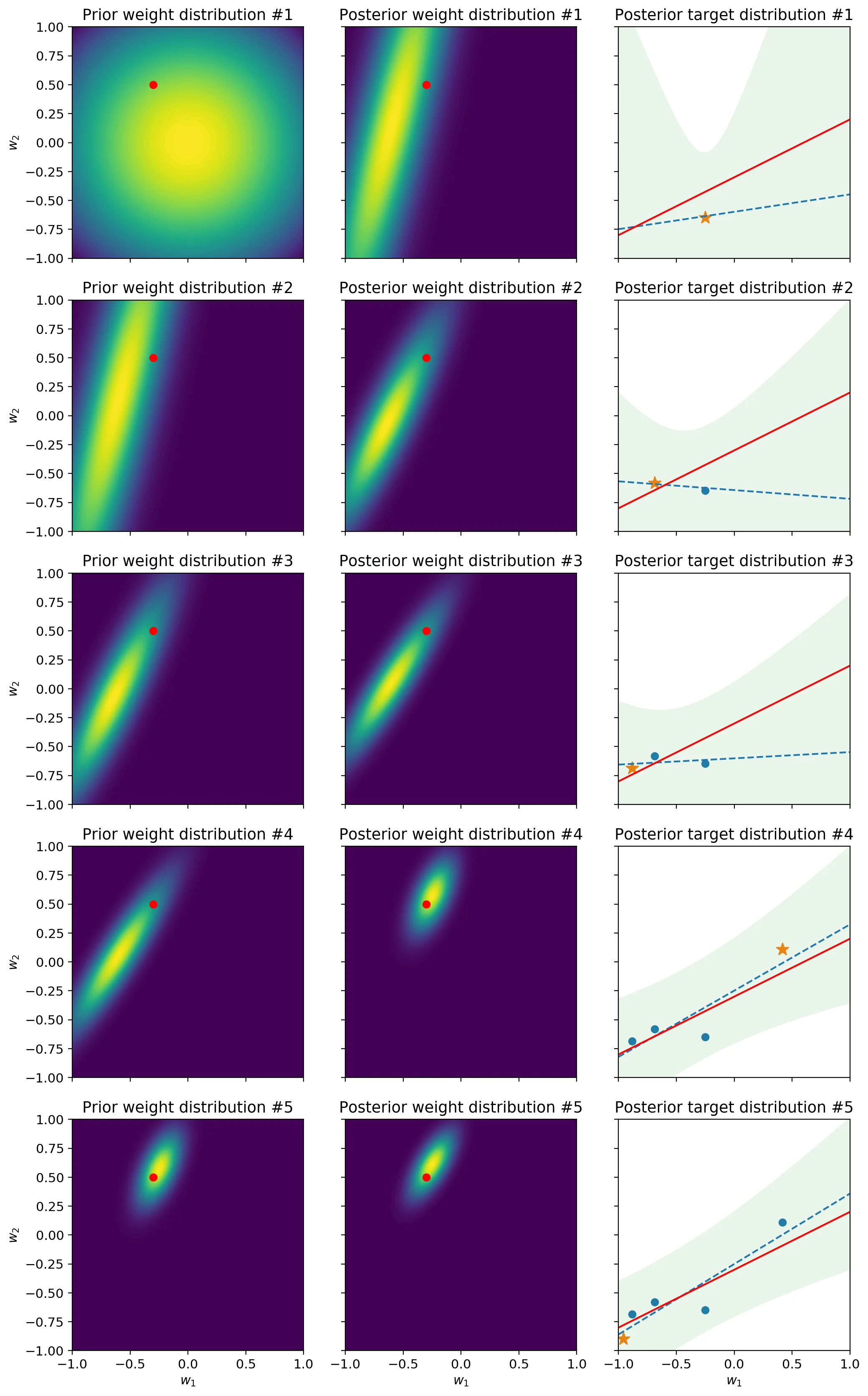
The first column represents the prior distribution of the weights. In other words, it shows what the model think the parameters should be, before seeing the next sample. The second column shows the distribution of the weights after the model has processed the next sample. In other words it represents the posterior distribution. You’ll notice that the prior distribution at each row is equal to the posterior distribution of the previous row. This stems from the fact that the posterior after having seen a sample becomes the prior for the next sample. Finally, the third column shows how this impacts the uncertainty of the posterior predictive distribution. Intuitively, as more samples arrive, the uncertainty lowers and the shaded area – which is a 95% predictive interval – becomes slimmer. Likewise, the fact that the ellipse representing the weight distribution shrinks indicates that the model is growing in confidence. As we will see later on, this isn’t always a good thing – hint: concept drift.
Prediction intervals
A nice property about Bayesian models is that they allow to quantify the uncertainty of predictions. In practical terms, the predict method of our implementation outputs a statistical distribution – to be precise, an instance of scipy.stats.norm. Therefore, we have access to an array of tools for free. For instance, we can use the interval method to obtain an interval in which it is likely that the prediction belongs. This interval, called the prediction interval, is a topic which confuses a lot of practitioners – including yours truly. I recommend reading this Wikipedia article to clarify your mind on the subject.
The thing to understand is that we’re using a parametric model, therefore the correctness of our prediction intervals is based on the assumption that the model choices we have made are valid. For instance, we are assuming that the likelihood follows a Gaussian distribution. Other models, such as gradient boosting, are non-parametric, and produce prediction intervals that are (almost) always reliable. Nonetheless, we can perform a visual check to see how reliable these prediction intervals actually are. To do so, we can check to see if the next target value is contained in the prediction interval. We can then calculate a running average of the amount of times where this occurs and display it along time. If we pick a confidence level of, say, 0.95, then we’re expecting to see around 95% of the predictions contained in the prediction interval. In the following snippet we’ll use the same sample method we used in the previous section.
np.random.seed(42)

model = BayesLinReg(n_features=2, alpha=1, beta=25)
pct_in_ci = 0
pct_in_ci_hist = []
n = 5_000

for i, (xi, yi) in enumerate(sample(n)):

    ci = model.predict(xi).interval(.95)
    in_ci = ci[0] < yi < ci[1]
    pct_in_ci += (in_ci - pct_in_ci) / (i + 1)  # online update of an average
    pct_in_ci_hist.append(pct_in_ci)

    model.learn(xi, yi)

fig, ax = plt.subplots(figsize=(9, 6))
ax.plot(range(n), pct_in_ci_hist)
ax.axhline(y=.95, color='red', linestyle='--')
ax.set_title('Quality of the prediction interval along time')
ax.set_xlabel('# of observed samples')
ax.set_ylabel('% of predictions in 95% prediction interval')
ax.set_ylim(.9, 1)
ax.grid()
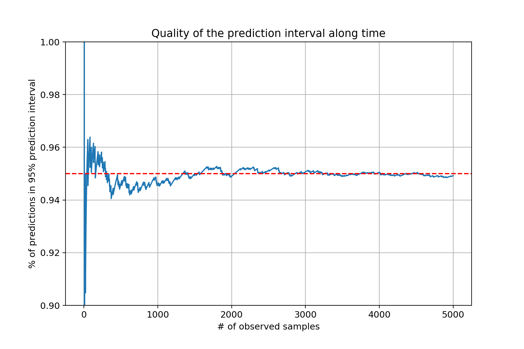
This seems to be working quite well; then again the generated data follows a Gaussian distribution so this was expected. What happens if try the same thing on a real-world dataset? As a test I’ve done exactly this on the California housing dataset, which is a moderately large dataset.
X, y = datasets.fetch_california_housing(return_X_y=True)

model = BayesLinReg(n_features=X.shape[1], alpha=1, beta=5)
pct_in_ci = 0
pct_in_ci_hist = []

for i, (xi, yi) in enumerate(zip(X, y)):

    ci = model.predict(xi).interval(.95)
    in_ci = ci[0] < yi < ci[1]
    pct_in_ci += (in_ci - pct_in_ci) / (i + 1)  # online update of an average
    pct_in_ci_hist.append(pct_in_ci)

    model.learn(xi, yi)

fig, ax = plt.subplots(figsize=(9, 6))
ax.plot(range(len(X)), pct_in_ci_hist)
ax.axhline(y=.95, color='red', linestyle='--')
ax.set_title('Quality of the prediction interval along time')
ax.set_xlabel('# of observed samples')
ax.set_ylabel('% of predictions in 95% prediction interval')
ax.grid()
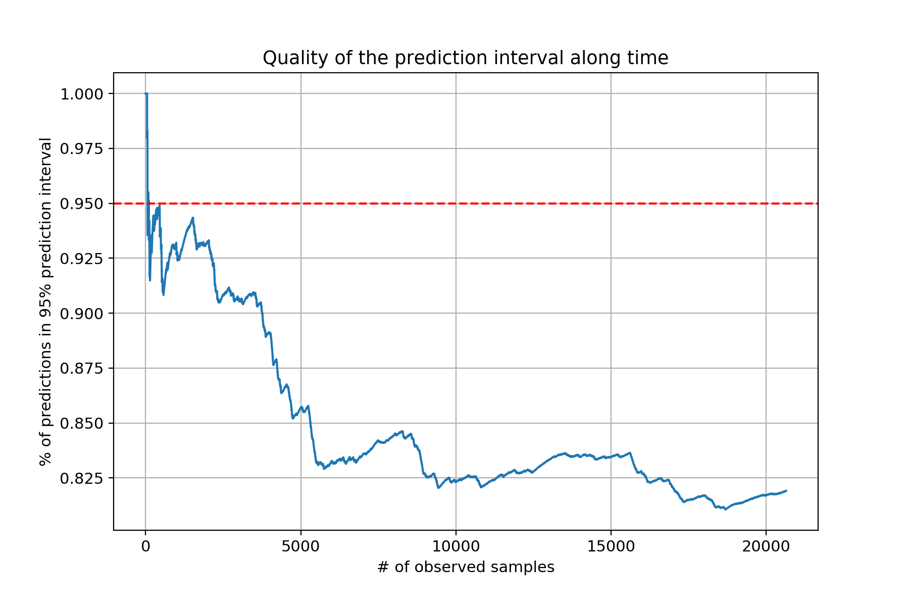
That definitely doesn’t look very good! That’s the problem with parametric models: they make assumptions about your data. If you’re really about prediction intervals that work regardless of your dataset – who wouldn’t want that? – then I would look into non-parametric prediction intervals and quantile regression – see for instance this GitHub issue for LightGBM.
Mini-batching
The main issue with our implementation of Bayesian linear regression is that it is horribly slow. The culprit is not hard the identify: it’s the matrix inversion we have to do at each step in order to update the inverse covariance matrix – actually in our specific implementation, a big chunk of time is spent creating instances of scipy.stats.norm, as explained in this GitHub issue, but that’s specific to this blog post. Indeed, the complexity of a matrix inversion is $\mathcal{O}(n^3)$ – actually, there seems to be an algorithm with complexity $\mathcal{O}(n^{2.373})$, but don’t ask me how it works. You have to understand that in most cases, people who use online machine learning use it to crunch huge datasets, therefore they very often resort to using algorithms that run in only $\mathcal{O}(n)$ time. For instance many practitioners use plain and simple stochastic gradient descent – albeit with a few bells and whistles. More sophisticated online optimizers have been proposed – such as the online Newton step, which uses the Hessian in addition to the gradient and runs in $\mathcal{O}(n^2)$ time – but are frowned upon because the name of the game is speed. Therefore, the complexity of our Bayesian linear regression, which has a lower bound complexity of $\mathcal{O}(n^3)$, is going to be a limiting factor for scaling to large datasets.
Later on, we’ll see how we can circumvent this issue by making different assumptions, but first I want to discuss mini-batching. I’m not going to go into the maths but it turns out that we can process multiple examples at the same time, whilst obtaining the same final model parameters. In other words, if process A and then B or A and B, the resulting model parameters will be exactly the same. This makes a lot of sense: you know the same amount of information whether I show you data piece by piece or all at the same time. The added benefit is that this significantly speeds up the learning step because it reduces the amount of matrix inversions which need to be performed.
We need to bring a few adjustments to our implementation in order to allow it to take in more than one observation at a time. We’ll make sure that the new implementation works for both a single pair $(x_i, y_i)$ as well as for a batch of pairs. This mostly boils down to numpy details that are not worth going into. I didn’t make these adjustments in the initial implementation in order to maximize readability. I am going to inherit from BayesLinReg in order not to have to copy/paste the __init__ method.
class BatchBayesLinReg(BayesLinReg):

    def learn(self, x, y):

        # If x and y are singletons, then we coerce them to a batch of length 1
        x = np.atleast_2d(x)
        y = np.atleast_1d(y)

        # Update the inverse covariance matrix (Bishop eq. 3.51)
        cov_inv = self.cov_inv + self.beta * x.T @ x

        # Update the mean vector (Bishop eq. 3.50)
        cov = np.linalg.inv(cov_inv)
        mean = cov @ (self.cov_inv @ self.mean + self.beta * y @ x)

        self.cov_inv = cov_inv
        self.mean = mean

        return self

    def predict(self, x):

        x = np.atleast_2d(x)

        # Obtain the predictive mean (Bishop eq. 3.58)
        y_pred_mean = x @ self.mean

        # Obtain the predictive variance (Bishop eq. 3.59)
        w_cov = np.linalg.inv(self.cov_inv)
        y_pred_var = 1 / self.beta + (x @ w_cov * x).sum(axis=1)

        # Drop a dimension from the mean and variance in case x and y were singletons
        # There might be a more elegant way to proceed but this works!
        y_pred_mean = np.squeeze(y_pred_mean)
        y_pred_var = np.squeeze(y_pred_var)

        return stats.norm(loc=y_pred_mean, scale=y_pred_var ** .5)
I’ll let you spot the differences if you are so inclined. In order to compare this with the original implementation, we’re going to split the California housing dataset in two – a training set and a test set.
from sklearn import model_selection

X, y = datasets.fetch_california_housing(return_X_y=True)
X_train, X_test, y_train, y_test = model_selection.train_test_split(
    X, y,
    test_size=.3,
    shuffle=True,
    random_state=42
)
First, let’s train the initial implementation on the training and compute it’s performance on the test set. I’m running this code in a Jupyter notebook so I have access to the %%time magic command to measure the execution time of the snippet.
%%time

model = BayesLinReg(n_features=X.shape[1], alpha=.3, beta=1)

for x, y in zip(X_train, y_train):
    model.learn(x, y)

y_pred = np.empty(len(X_test))

for i, (x, _) in enumerate(zip(X_test, y_test)):
    y_pred[i] = model.predict(x).mean()

print(metrics.mean_absolute_error(y_test, y_pred))
This produces a mean absolute error of around 0.57, and takes approximatively 4.66s to run. Now let’s run our newly implemented BatchBayesLinReg and feed it all the training set at once.
%%time

model = BatchBayesLinReg(n_features=X.shape[1], alpha=.3, beta=1)

model.learn(X_train, y_train)
y_pred = model.predict(X_test).mean()

print(metrics.mean_absolute_error(y_test, y_pred))
As expected, this outputs a mean absolute error of around 0.57, which is identical to the online version. However, the execution time is now only a mere 6.42ms, which is a whopping 725 times faster! Therefore the only advantage of the streaming variant is that it allows you to not have to retrain the model when new data is available. The twist is that we can use the best of both worlds: we can “warm-start” our model by training on a big batch of data, and afterwards feed it individual samples. Bayesian models are really flexible that way. The “only” downside of the batch approach is that it requires having all the data available at once. In some contexts this isn’t feasible nor desirable. As a compromise, we can train the model with mini-batches by chunking the training set into batches of, say, 16 observations:
%%time

model = BatchBayesLinReg(n_features=X.shape[1], alpha=.3, beta=1)

batch_size = 16
n_batches = len(X_train) // batch_size

batches = zip(
    np.array_split(X_train, n_batches),
    np.array_split(y_train, n_batches)
)

for x_batch, y_batch in batches:
    model.learn(x_batch, y_batch)

y_pred = model.predict(X_test).mean()

print(metrics.mean_absolute_error(y_test, y_pred))
This produces the same mean absolute error, and takes 36.9ms to execute, which is 126 times faster than the online variant.
Handling concept drift
Concept drift occurs when something in the data generating process changes. A common assumption of machine learning models is that the data the model will encounter after it’s training phase – call it the test set, if you like – has the same statistical properties as the training set. If this assumption is violated, then the model is bound to underperform. In practice, when you deploy a machine learning model, the model’s performance will usually degrade along time because “something” in the data is changing. If you want to read more about concept drift, I recommend reading the Wikipedia article on the topic, it has some nice real-world examples in it.
Most practictioners use batch machine learning; they therefore deal with concept drift by retraining the model as often as possible. As you can imagine, this isn’t very efficient and consumes a lot of resources. Meanwhile, a good online machine model can and should be able to handle concept drift. This guarantees that it’s performance remains stable along time. Let’s see if our BayesLinReg implementation is able to cope with concept drift. As a benchmark, I’ve decided to simulate a concept drift. There are datasets out there that contain concept drift, but I wanted to have fine-grained control on the data generating process. I decided on something relatively simple: I picked two sets of linear regression parameters, and slowly transitioned from one to the other. I’m sure there’s a nice way to write this mathematically, but I believe that the code speaks for itself:
def sample(first_period=100, transition_period=50, second_period=100):

    # Pick two pairs of weights which the model is going to have to find
    start_weights = np.array([-.3,  .5])
    end_weights   = np.array([  1, -.7])

    for i in range(first_period + transition_period + second_period):

        # Sample a vector of features
        x = np.array([1, np.random.uniform(-1, 1)])

        # Decide which set of weights to use
        if i < first_period:
            weights = start_weights

        elif i < first_period + transition_period:
            ratio = (i - first_period) / transition_period
            weights = ratio * start_weights + (1 - ratio) * end_weights

        else:
            weights = end_weights

        # Yield the features and the target (with some noise)
        yield x, np.dot(weights, x) + np.random.normal(0, .2)
For the first first_period steps, the sample function generates samples using the first set of weights. For the last second_period steps, it uses the second set of weights. In between, it mixes both sets of weights together depending on the number of the iteration. Let’s see if this is able to trick our model.
np.random.seed(42)
model = BayesLinReg(n_features=2, alpha=2, beta=25)
y_true = []
y_pred = []
first_period = 100
transition_period = 50
second_period = 100
for i, (xi, yi) in enumerate(sample(first_period, transition_period, second_period)):
y_true.append(yi)
y_pred.append(model.predict(xi).mean())
model.learn(xi, yi)
# Convert to numpy arrays for comfort
y_true = np.array(y_true)
y_pred = np.array(y_pred)
score = metrics.mean_absolute_error(y_true, y_pred)
fig, ax = plt.subplots(figsize=(9, 6))
ax.scatter(
range(len(y_true)), np.abs(y_true - y_pred),
marker='|', label='Individual absolute errors'
)
ax.plot(
np.cumsum(np.abs(y_true - y_pred)) / (np.arange(len(y_true)) + 1),
color='red', label='Running average of the error'
)
ax.axvspan(
first_period, first_period + transition_period,
alpha=.1, color='green', label='Transition period'
)
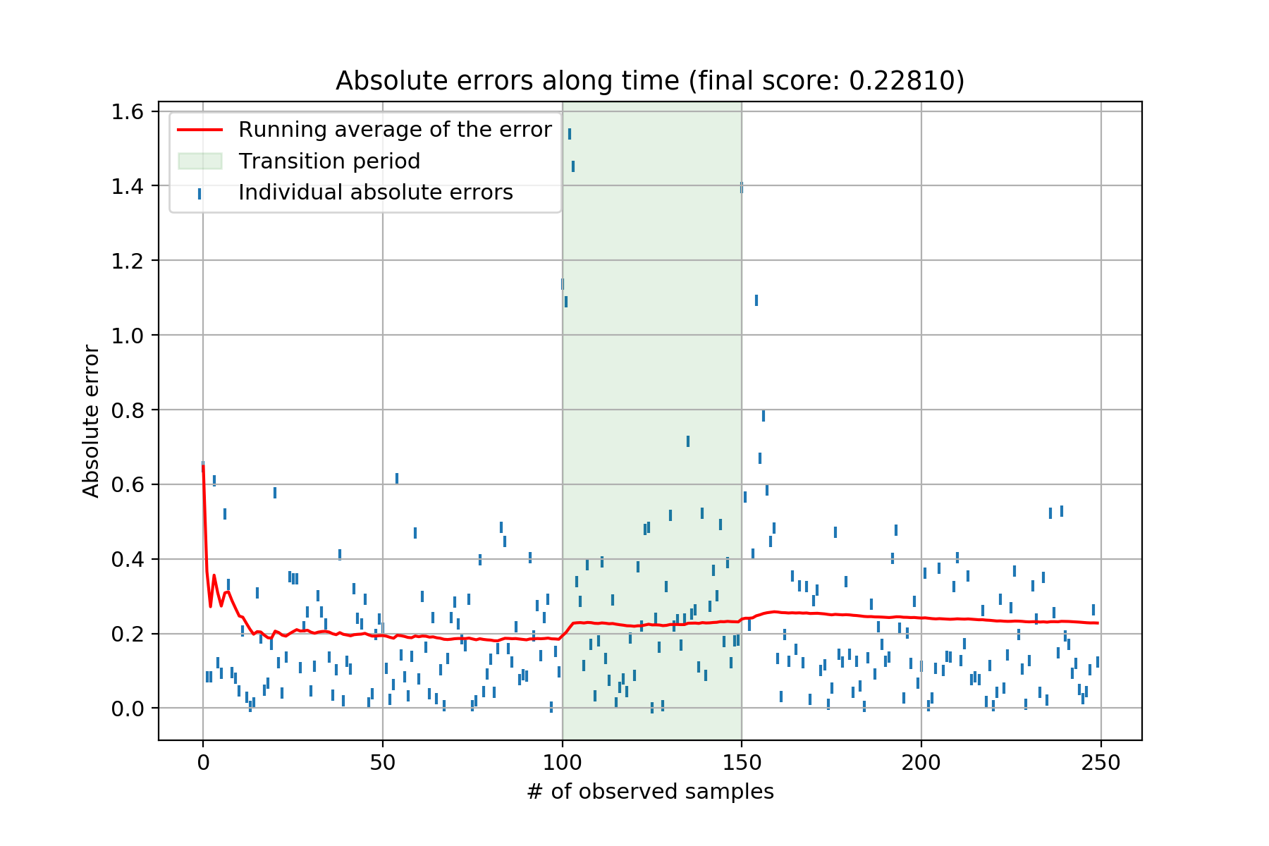
ax.set_title(f'Absolute errors along time (final score: {score:.5f})')
ax.set_xlabel('# of observed samples')
ax.set_ylabel('Absolute error')
ax.legend()
ax.grid()
This produces the following chart:
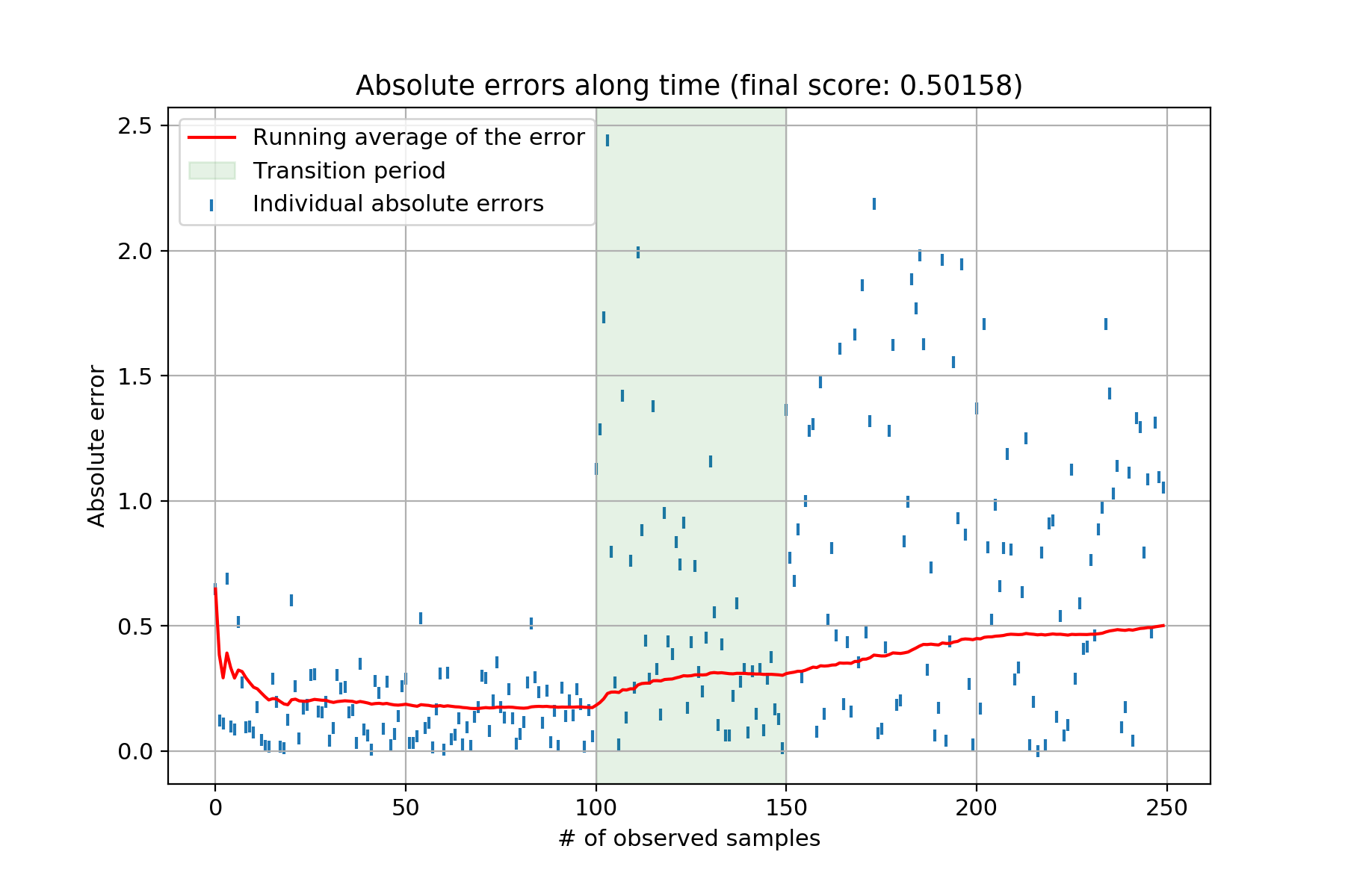
Each individual blue tick represents the absolute error between the ground truth and the model’s estimate. The red line is the running average of said errors. The green shaded area represents the transition period between both sets of weights the model has to uncover. Clearly, once the data generating starts changing – i.e., the beginning of the green shaded area – the model’s performance starts to deteriorate. The Bayesian linear regression therefore isn’t coping very well with concept drift. Can we do something about it? I’ve never seen this answered in textbooks. The only place I found something mentionned about it was in Vincent Warmerdam’s blog post – in the Extra Modelling Options section. He hints at using a smoothing factor to essentially give more importance to recent observations. As he says, this feels a bit like a hack, mostly because there doesn’t seem to be much theoretical justification to back this “trick”. Nonetheless, I tinkered with Vincent’s idea and it seems to work rather well. Here goes:
class RobustBayesLinReg(BayesLinReg):

    def __init__(self, smoothing, n_features, alpha, beta):
        super().__init__(n_features, alpha, beta)
        self.smoothing = smoothing

    def learn(self, x, y):

        # Update the inverse covariance matrix, with smoothing
        cov_inv = (
            self.smoothing * self.cov_inv +
            (1 - self.smoothing) * self.beta * np.outer(x, x)
        )

        # Update the mean vector, with smoothing
        cov = np.linalg.inv(cov_inv)
        mean = cov @ (
            self.smoothing * self.cov_inv @ self.mean +
            (1 - self.smoothing) * self.beta * y * x
        )

        self.cov_inv = cov_inv
        self.mean = mean

        return self
I’ll let you compare this with the initial implementation. In terms of update equations, by denoting with $\gamma$ the smoothing factor, this is what it looks like:
$$S_{i+1} = (\gamma S_i^{-1} + (1 - \gamma)\beta x_i^\intercal x_i)^{-1}$$
$$m_{i+1} = S_{i+1}(\gamma S_i^{-1} m_i + (1 - \gamma) \beta x_i y_i)$$
Note that in the new implementation nothing changes for the predict method; we’ve therefore inherited from BayesLinReg to avoid an unnecessary copy/paste. The smoothing works essentially like an exponentially weighted average – as a reference, see the alpha parametrisation of the ewm method in pandas. Let’s check out the performance of this model on the same scenario when using a smoothing factor of 0.8 – which is actually the only value I tried because it worked.
Click to see the code
np.random.seed(42)

model = RobustBayesLinReg(smoothing=.8, n_features=2, alpha=2, beta=25)

y_true = []
y_pred = []

for i, (xi, yi) in enumerate(sample(first_period, transition_period, second_period)):
    y_true.append(yi)
    y_pred.append(model.predict(xi).mean())
    model.learn(xi, yi)

# Convert to numpy arrays for comfort
y_true = np.array(y_true)
y_pred = np.array(y_pred)

score = metrics.mean_absolute_error(y_true, y_pred)

fig, ax = plt.subplots(figsize=(9, 6))
ax.scatter(
    range(len(y_true)), np.abs(y_true - y_pred),
    marker='|', label='Individual absolute errors'
)
ax.plot(
    np.cumsum(np.abs(y_true - y_pred)) / (np.arange(len(y_true)) + 1),
    color='red', label='Running average of the error'
)
ax.axvspan(
    first_period, first_period + transition_period,
    alpha=.1, color='green', label='Transition period'
)
ax.set_title(f'Absolute errors along time (final score: {score:.5f})')
ax.set_xlabel('# of observed samples')
ax.set_ylabel('Absolute error')
ax.legend()
ax.grid()
It seems to be working very well! Some would say this is worth writing a research paper. I’m sure that there’s already one that exists, but I haven’t found it yet.
Zero mean isotropic Gaussian prior

This section title is a bit of a mouthful – at least for me – but it’s actually simpler than it sounds. In his book, Christopher Bishop proposes a simpler prior distribution for the weights which significantly reduces the amount of computation to perform. Under this prior, which is still a $p$-dimensional Gaussian, the weights are centered around 0 – hence the “zero mean” – whilst they each have the same variance – which corresponds to the “isotropic” part. Mathematically, the prior is defined as so:
$$\begin{equation} \color{royalblue} p(w_0) = \mathcal{N}(0, \alpha^{-1}I) \end{equation}$$
This leads to the following posterior distribution for the weights:
$$\begin{equation} \color{mediumpurple} p(w_{i+1} | w_i, x_i, y_i) = \mathcal{N}(m_{i+1}, S_{i+1}) \end{equation}$$
$$\begin{equation} S_{i+1} = (\alpha I + \beta x_i^\intercal x_i)^{-1} \end{equation}$$
$$\begin{equation} m_{i+1} = \beta S_{i+1} x_i^\intercal y_i \end{equation}$$
At a first glance, these formulas look just as heavy as before because they still necessitate a matrix inversion. The trick is that the equation for obtaining $S_{i+1}$ has a particular structure that we can exploit. Indeed, it turns out that there is a wonderful formula to evaluate this equation without having to explicitely apply the inverse operation – I love it when this happens. It’s called the Sherman–Morrison formula. Here it is with Wikipedia’s notation:
$$\begin{equation} (A + uv^\intercal)^{-1} = A^{-1} - \frac{A^{-1} uv^\intercal A^{-1}}{1 + v^\intercal A^{-1}u} \end{equation}$$
In our case, we have:
$$\begin{equation} A \leftarrow \alpha I \end{equation}$$
$$\begin{equation} u \leftarrow x \end{equation}$$
$$\begin{equation} v \leftarrow x \end{equation}$$
This formula is efficient because we only have to compute $A^{-1}$ once. The following snippet contains the implementation of Bayesian linear regression with a zero mean isotropic Gaussian prior and the Sherman-Morrisson formula:
def sherman_morrison(A_inv, u, v):
    num = A_inv @ np.outer(u, v) @ A_inv
    den = 1 + v @ A_inv @ u
    return A_inv - num / den


class SimpleBayesLinReg:

    def __init__(self, n_features, alpha, beta):
        self.n_features = n_features
        self.alpha = alpha
        self.beta = beta
        self.mean = np.zeros(n_features)
        self.A_inv = np.linalg.inv(alpha * np.identity(n_features))
        self.cov = self.A_inv

    def learn(self, x, y):

        # Update the inverse covariance matrix (Bishop eq. 3.54)
        self.cov = sherman_morrison(A_inv=self.A_inv, u=self.beta * x, v=x)

        # Update the mean vector (Bishop eq. 3.53)
        self.mean = self.beta * self.cov @ x * y

        return self

    def predict(self, x):

        # Obtain the predictive mean (Bishop eq. 3.58)
        y_pred_mean = x @ self.mean

        # Obtain the predictive variance (Bishop eq. 3.59)
        y_pred_var = 1 / self.beta + x @ self.cov @ x.T

        return stats.norm(loc=y_pred_mean, scale=y_pred_var ** .5)
Let’s apply progressive validation with the Boston housing dataset.
X, y = datasets.load_boston(return_X_y=True)

model = SimpleBayesLinReg(n_features=X.shape[1], alpha=.3, beta=1)

y_pred = np.empty(len(y))

for i, (xi, yi) in enumerate(zip(X, y)):
    y_pred[i] = model.predict(xi).mean()
    model.learn(xi, yi)

print(metrics.mean_absolute_error(y, y_pred))
This produces a mean absolute error of around 4.6. For reference the initial implementation scored 3.78, so this new model isn’t as good.
Conclusion
That wraps it up for now. There are definitely some more directions I would like to take, namely:
- Supporting binary and multi-class classification: this would require determining other update formulas, probably based on a binomial distribution for the likelihood function.
- Learning
alphaandbeta: in his book, Christopher Bishop points at some ways to estimate both hyperparameters from the data. However, I need to drink a lot more coffee in order to understand how he proceeds. - Handling sparse feature vectors: it would be nice to handle a large number features by allowing sparse computation (and not just manually filling the gaps of
xwith 0s!). This would lead the way, for instance, to Bayesian factorisation machines – although that already seems to be something. - Non-zero mean isotropic Gaussian prior: the prior introduced in the last section doesn’t perform as well as the initial implementation; I wonder if it’s possible to specify a model somewhere in between and therefore obtain a better whilst still avoiding to have to compute a matrix inversion at every iteration.
- Implementing a “master class” where all the variants and tricks I have presented are implemented and can be switched on or off.
I will eventually dig into these topics. My initial plan was to include them in this post, but I’ve been waiting to publish this post for far too long – plus it’s already quite dense. If this post has peaked your interest and you would like to collaborate or have some questions, then feel free to get in touch with me at maxhalford25@gmail.com. Also, I’ve put all the code used in this blog post and put it in this gist. The next step for me is going to be to implement Bayesian linear regression in creme, which is an online machine learning library I maintain.