Halftoning with Go - Part 2

The next stop on my travel through the world of halftoning will be the implementation of Weighted Voronoi Stippling as described in Adrian Secord’s 2002 paper. This method is more involved than the ones I detailed in my previous blog post, however the results are quite interesting. Again, I did the implementation in Go.

Overview

I found a fair amount of resources about the method, most of them being implementations of Adrian Secord’s paper. However, not many of these resources went into the nitty-gritty details which are not obvious for beginners in image processing. Before delving into the code, I want to go through some concepts that may seem obvious to some readers but that I judge worthy of detailing.

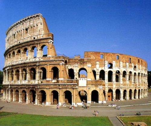
In art, stippling is a process where single-colored dots are laid out on a white image so as to reproduce an image. The denser the dots, the darker the area they cover. The visual appeal of stippled images comes from the way the dots are laid out. A good stippling method generates evenly spaces dots which makes the image seem organized. This kind of harmonious distribution is often referred to as blue noise and is notoriously difficult to generate.

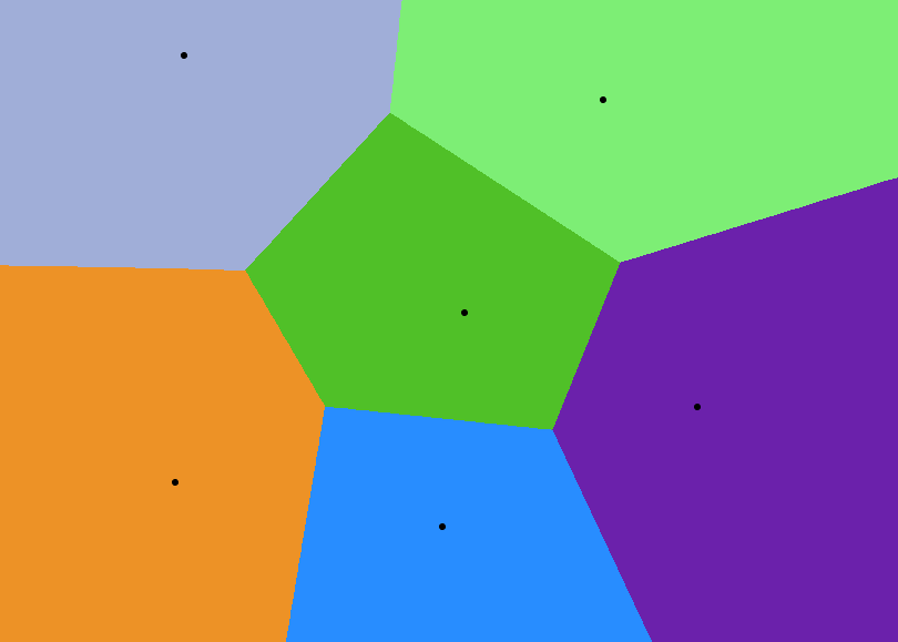
Adrian Secord’s idea - inspired Oliver Deussen’s previous work from 2000 - is to use weighted centroidal Voronoi diagrams to place the dots. Although the name may seem far fetched, the underlying idea is very simple and can be broken down into three parts.

Voronoi diagrams (also called Voronoi tessellations) are a huge topic and are surprisingly used in many areas of research. A Voronoi diagram consists of a number of sites and regions. To each site there belongs a region wherein each point has a shorter distance to the site than it does to any other site. In an image, the sites would a list of $(x, y)$ pairs with discrete coordinates; to generate the Voronoi diagram we would iterate over each pixel in the image, calculate the distance to each site and then assign each pixel to the site to which it is closest. This is one of way of generating Voronoi diagrams, however it obliges us to use integers which isn’t very handy when doing fine-grained image processing. A Voronoi diagram can also be seen as a set of vertices and edges which can be obtained by using Fortune’s algorithm. As we will see this representation doesn’t suit our purpose and we have to stick to the sites/regions representation. I’ll detail the method I used in a further section.

A Centroidal Voronoi diagram is a Voronoi diagram where the sites are at the centroid of their respective region. Because each region is a polygon, their exists a formula for calculating the centroids by looking at the vertices. However, a more intuitive way of calculating a polygon centroid is:

$$c_x = \frac{1}{|S|} \int_S x dS$$

$$c_y = \frac{1}{|S|} \int_S y dS$$

where $c_x$ and $c_y$ are respectively the $x$ and $y$ coordinates of a polygon defined by a set of points $S$. In English we are simply taking the average $x$ and $y$ coordinates as the centroids. We gain in simplicity what we lose in speed; the formula using the vertices is much faster. In our case we are dealing with images and discrete values; sums have to be used instead of integrals.

$$c_x = \frac{1}{|S|} \sum_{p \in S} p(x)$$

$$c_y = \frac{1}{|S|} \sum_{p \in S} p(y)$$

Producing a centroidal Voronoi diagram requires iterating the following steps:

1. Calculate each region’s centroid
2. Move the sites to their corresponding centroid
3. Reassign the points to their closest site

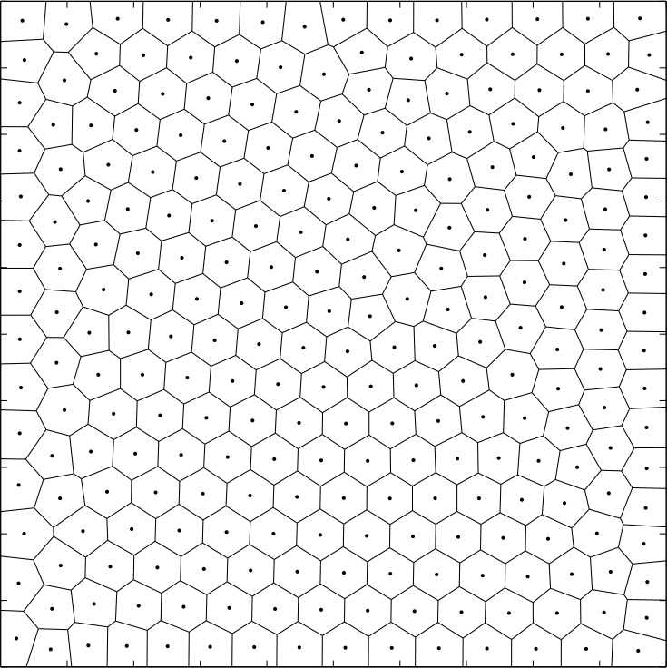
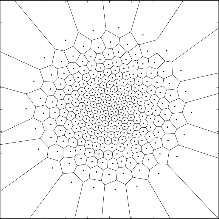
This procedure is called Lloyd’s algorithm and is used in other algorithms just as k-means clustering. As can be seen in the following image, after a few iterations - usually 15 does the trick - the regions start to have the same shape and size and seem to organize themselves.

A weighted centroidal diagram is a centroidal Voronoi diagram where the centroids are calculated using a weighted average. In our case the weights are the gray scale intensities of an image. The idea is that we want the centroids to bundle around dark patches of an image and yet not to overlap. That’s it, there is nothing more it; the results speak for themselves. The previous formulas are easy to adapt:

$$c_x = \frac{1}{W \times |S|} \sum_{p \in S} p(w) \times p(x)$$

$$c_y = \frac{1}{W \times |S|} \sum_{p \in S} p(w) \times p(y)$$

where $W = \sum_{p \in S} p(w)$. If this isn’t clear bear with me until we get to the implementation, everything will seem clearer.

The following image was produced by using an gray scale image of a blank image with a circle in the center. By taking into account the gray scale values, the centroids move towards the center whilst remaining somewhat “organized”.

Now for the implementation!

Importance sampling

An initial set of points is required for generating a Voronoi diagram. What’s more, it would be nice to be able to control the number of points used for stippling. A simple solution is to sample a set of points completely at random. Although this works, it means that more iterations will be required to converge onto a weighted centroidal Voronoi diagram. A smarter way of doing is to sample points with a distribution based on the gray scale intensities of an image. In other words to sample more points where the image is dark and less where the image is light. This way of doing is called importance sampling because the darker pixels - the dark ones - will be sampled more that the light ones.

My implementation is inspired from the roulette wheel selection algorithm used in genetic algorithms:

1. Created a weighted roulette with decreasing pocket sizes and one pocket per gray scale intensity
2. Choose a random number between 0 and the sum of the pocket sizes
3. See in which pocket the random number falls
4. Pick a random point with the obtained intensity

In our case the gray scale intensities go from 0 to 255, hence we will have 256 pockets. If we picked a random number between 0 and 255 then we would be picking intensities completely at random. We want to pick darker intensities more often, hence we are going to “weight” the pockets with the intensities. This is quite simple, each pocket will simply have a size/weight of $256 - i$ where $i$ is the intensity; this way the darker intensities - the ones closer to 0 - will have a higher waits.

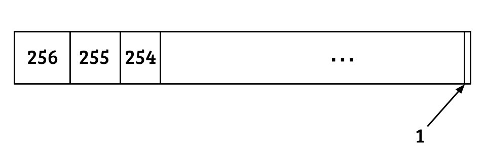
To be able to “run” the wheel we need to generate numbers and see in which pocket they lie. To do so we have to generate a cumulative roulette wheel and generate a random number between 0 and the last roulette wheel value.

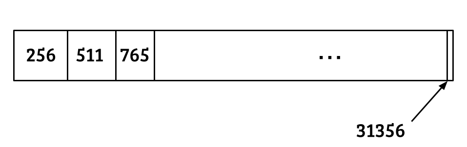
The code for creating the cumulative roulette wheel is quite simple.

var roulette = make([]int, 256)
roulette[0] = 256
for i := 1; i < len(roulette); i++ {
    roulette[i] = roulette[i-1] + (256 - i)
}

We also need some sort of data structure to map intensities to matching points. This can simply be a hash table where the keys are the intensities and the values are the belonging points.

var (
    bounds = gray.Bounds()
    hist   = make(map[uint8]Points)
)
for x := bounds.Min.X; x < bounds.Max.X; x++ {
    for y := bounds.Min.Y; y < bounds.Max.Y; y++ {
        var intensity = gray.GrayAt(x, y).Y
        hist[intensity] = append(hist[intensity], Point{float64(x), float64(y)})
    }
}

In the above snippet gray is an image.Image from Go’s standard library. The Point struct is a custom one where the coordinates are floating point numbers. Go’s image.Point doesn’t suit our particular needs because it’s coordinates are integers.

type Point struct {
    X float64
    Y float64
}

The final step is to generate random numbers and see in which pocket they lie. Once we generate a number, we could simply iterate through the roulette wheel and check for the first index whose value is above the generated number. However the values in our roulette wheel are sorted, hence we can use binary search to speed things up. Conveniently Go’s standard library contains a sort.Search method which does exactly what we need; a sort.SearchInts convenience method even exists. The following snippet contains my final implementation of importance sampling.

func ImportanceSample(n int, gray *image.Gray, threshold uint8, rng *rand.Rand) Points {
    var (
        pts    = make(Points, n)
        bounds = gray.Bounds()
        hist   = make(map[uint8]Points)
    )
    // Build a histogram
    for x := bounds.Min.X; x < bounds.Max.X; x++ {
        for y := bounds.Min.Y; y < bounds.Max.Y; y++ {
            var intensity = gray.GrayAt(x, y).Y
            if intensity <= threshold {
                hist[intensity] = append(hist[intensity], Point{float64(x), float64(y)})
            }
        }
    }
    // Build a roulette wheel
    var roulette = make([]int, threshold+1)
    roulette[0] = 256
    for i := 1; i < len(roulette); i++ {
        roulette[i] = roulette[i-1] + (256 - i)
    }
    // Run the wheel
    for i := range pts {
        var (
            ball = rng.Intn(roulette[len(roulette)-1])
            bin  = sort.SearchInts(roulette, ball)
            p    = hist[uint8(bin)][rng.Intn(len(hist[uint8(bin)]))]
        )
        p.X += rng.Float64()
        p.Y += rng.Float64()
        pts[i] = p
    }
    return pts
}

We want to generate n points which we store in a slice called pts. We start by building a hash table mapping each intensity to a set of matching of points. I added a threshold parameter so that higher intensities - the ones closer to white - are discarded. Next we build the roulette wheel; because of the threshold parameter the values above it are not taken into account in the roulette wheel. Finally we generate a random number - called ball - and we use sort.SearchInts to obtain the intensity from which to sample a random point p in the hash table hist. I added some noise to the sampled points in case a point is sampled twice. Here is an example of applying the method with a sample of size 10000.

I don’t want to spend more time going through the intricacies of importance sampling because it is a bit off topic. If you’re interested I’ve added the method to the halfgone package. The main idea to take away is that I wanted a method that could produce a fixed number of points with a distribution somewhat reproducing the darkness of the image. If you want to implement Weighted Voronoi Stippling yourself, you’ll do just fine by generating a initial set of points completely at random!

Using a kd-tree for computing Voronoi diagrams

Now that we have an initial set of points, we are going to use Lloyd’s algorithm for “relaxing” the points in a harmonious disposition. However, to do so we need to be able to build a Voronoi diagram because the relaxation step involves points towards their Voronoi region centroid.

As mentioned earlier, obtaining the vertices and edges that define a Voronoi diagram isn’t enough if we want to compute weighted centroids. We need to be able to know the coordinates and the weights of each point belonging to a region to be able to calculate it’s region. A naive way of doing is to iterate through each point of an image and to determine it’s closest site by calculating the distance towards each site. This is called nearest neighbour search and is a well known problem in computer science; there are many data structures that make it possible to save a lot of time.

I settled on using a kd-tree; I don’t want to delve into it too far because there are already many existing resources online. I based myself on this tutorial from Carnegie Mellon. I used three Go structs for the implementation.

type rectangle struct {
    min, max Point
}

type kdNode struct {
    p           Point
    splitByX    bool
    left, right *kdNode
}

type kdTree struct {
    root   *kdNode
    bounds rectangle
}

The rectangle struct represents the “boxes” the kd-tree splits a two-dimensional into. A kdNode is an element of a kdTree and represents a splitting point. The splitByX field indicates if the node partitions the space in two left and right rectangles or two top and bottom ones. In a generic implementation the kd-tree would be applied to a multi-dimensional and splitByX would be replaced by an integer to indicate which dimension the split is applied to. The kd-tree algorithms has two phases: the building and the searching, in my implementation both are recursive.

The building part is the easiest part. Say we have a list of points $S$ and we want to build a kd-tree on top of it. We start with a dimension at random, for example the $x$-axis. The only thing we have to do is to find the point with the median $x$ value; this is easily done by sorting $S$ according to each points $x$ value and then choosing the value at the middle of the $S$. The point is then added to the kd-tree and we run the same thing we just did on the halves that were produced, hence the recursion I mentioned. The reason why median points are chosen can be understood from a heuristic point of view: having boxes more or less of the same size will narrow down the search space faster.

func makeKdTree(pts Points, bounds rectangle) kdTree {

    var split func(pts Points, splitByX bool) *kdNode

    split = func(pts Points, splitByX bool) *kdNode {

        if len(pts) == 0 {
            return nil
        }

        if splitByX {
            pts.sortByX()
        } else {
            pts.sortByY()
        }

        med := len(pts) / 2

        return &kdNode{
            p:        pts[med],
            splitByX: splitByX,
            left:     split(pts[:med], !splitByX),
            right:    split(pts[med+1:], !splitByX),
        }

    }

    return kdTree{
        root:   split(pts, true),
        bounds: bounds,
    }
}

The points are either sorted along the $x$-axis by calling pts.sortByX or along the $y$-axis with pts.sortByY depending on the value of splitByX. Here is the code for sortByX:

func (pts Points) sortByX() {
    sort.Slice(pts, func(i, j int) bool { return pts[i].X < pts[j].X })
}

Go can be a nice language, right? The median value is then obtained by dividing the length of the list of points and rounding it down with med := len(pts) / 2. Finally we call the split on each sub-list by slicing the original list on med.

The search phase is bit more complex and I don’t want to go into it in detail, it’s already quite well explained from page 6 in the Carnegie Mellon tutorial. Basically, the search starts by doing a depth-first search for the closest leaf node to the target point. As the tutorial explains, this is already a good approximation. However, if the circle with a radius equal to distance between the target point and the lead node overlaps the parent node’s box, then the algorithms goes up a level and checks other branches for closer points. It’s fine if you don’t know how kd-trees work, the only thing to remember is that they are a data structure that allows us to search for nearest neighbours in a timely fashion. Nevertheless, here is the Go code for performing a search.

func (t kdTree) findNearestNeighbour(p Point) (best Point, bestSqd float64) {

    var search func(node *kdNode, target Point, r rectangle, maxDistSqd float64)
    (nearest Point, distSqd float64)

    search = func(node *kdNode, target Point, r rectangle, maxDistSqd float64)
    (nearest Point, distSqd float64) {

        if node == nil {
            return Point{}, math.Inf(1)
        }

        var targetInLeft bool
        var leftBox, rightBox rectangle
        var nearestNode, furthestNode *kdNode
        var nearestBox, furthestBox rectangle

        if node.splitByX {
            leftBox = rectangle{r.min, Point{node.p.X, r.max.Y}}
            rightBox = rectangle{Point{node.p.X, r.min.Y}, r.max}
            targetInLeft = target.X <= node.p.X
        } else {
            leftBox = rectangle{r.min, Point{r.max.X, node.p.Y}}
            rightBox = rectangle{Point{r.min.X, node.p.Y}, r.max}
            targetInLeft = target.Y <= node.p.Y
        }

        if targetInLeft {
            nearestNode, nearestBox = node.left, leftBox
            furthestNode, furthestBox = node.right, rightBox
        } else {
            nearestNode, nearestBox = node.right, rightBox
            furthestNode, furthestBox = node.left, leftBox
        }

        nearest, distSqd = search(nearestNode, target, nearestBox, maxDistSqd)
        if distSqd < maxDistSqd {
            maxDistSqd = distSqd
        }

        var d float64
        if node.splitByX {
            d = node.p.X - target.X
        } else {
            d = node.p.Y - target.Y
        }
        d *= d

        if d > maxDistSqd {
            return
        }

        if d = node.p.getDist(target); d < distSqd {
            nearest = node.p
            distSqd = d
            maxDistSqd = distSqd
        }

        tmpNearest, tmpSqd := search(furthestNode, target, furthestBox, maxDistSqd)
        if tmpSqd < distSqd {
            nearest = tmpNearest
            distSqd = tmpSqd
        }
        return
    }

    return search(t.root, p, t.bounds, math.Inf(1))
}

Point relaxation

The last piece of the puzzle is implementing Lloyd’s algorithm for relaxing the points obtained after importance sampling. First of all we are going to generate a 2D probability density function (PDF) to determine the tone distribution on a given image. We will be using the PDF to “weight” the centroids calculations. Generating a PDF from an image is trivial.

// A PDF is a probability density function.
type PDF [][]float64

// makePDF generates a probability density function from an image.Gray.
func MakePDF(gray *image.Gray) PDF {
    var (
        bounds = gray.Bounds()
        pdf    = make(PDF, bounds.Dx())
    )
    for x := 0; x < bounds.Dx(); x++ {
        pdf[x] = make([]float64, bounds.Dy())
        for y := 0; y < bounds.Dy(); y++ {
            pdf[x][y] = 255 - float64(gray.GrayAt(x, y).Y)
        }
    }
    return pdf
}

Our PDF is simply a 2D matrix where each cell corresponds to 255 minus the underlying gray intensity - so that darker values have higher values in the PDF. Usually a PDF has to sum up to 1 - this can be done by dividing each cell in the matrix by it’s total sum - however for our purposes this isn’t necessary.

We are going to be using three intermediate containers for storing information about the centroids.

var (
    siteCentroids = make(map[Point]Point)
    siteDensities = make(map[Point]float64)
    siteAreas     = make(map[Point]float64)
)

siteCentroids is going to map each site to it’s centroid. The idea being that once the centroids are obtained they become the sites and new centroids can be calculated. siteIntensities is going to contain the total gray intensities associated to each site, which will be used for calculating the centroids and for adjusting the point sizes during rendering - I’ll get to this later. For the moment let’s look at the following piece of code.

for i := box.min.X; i < box.max.X; i += step {
    for j := box.min.Y; j < box.max.Y; j += step {
        p := Point{i, j}
        nn, _ := kd.findNearestNeighbour(p)
        w := pdf[int(i)][int(j)]
        centroid := siteCentroids[nn]
        centroid.X += w * p.X
        centroid.Y += w * p.Y
        siteCentroids[nn] = centroid
        siteIntensities[nn] += w
        siteNPoints[nn]++
    }
}

For calculating the centroids we have to calculate a weighted sum of each point contained in a Voronoi region. To do so I looped through each cell of the image, found it’s closest site and then added the $x$ and $y$ coordinates to the matching centroid. In the previous snippet box is a rectangle which I defined earlier, I initialize one for generating the kd-tree associated to the input image bounds and the given sites.

var (
    box = rectangle{
        Point{float64(bounds.Min.X), float64(bounds.Min.Y)},
        Point{float64(bounds.Max.X), float64(bounds.Max.Y)},
    }
    kd = makeKdTree(sites, box)
)

At first I incremented i and j, this seemed but my final images were very blurry. It took me a fair amount of time to realize that I was lacking granularity and that Voronoi regions which were smaller than a pixel were getting overwritten. It’s a bit difficult to understand but Adrian Secord mentions it in his paper, he refers to this paper for the solution. The trick is to increase the virtual resolution of the image and calculate the centroids with more points. I didn’t find any implementations so maybe I’m wrong but my understanding is that this means that we should increment i and j with a smaller step than 1. I chose to add a resolution parameter to my algorithm and I define step to be 1 / resolution. This means that for a resolution value of 4 the algorithm iterates through $4^2 = 16$ more values than by default - the height and the width are each increased by 4. As I iterate through the image I also store the underlying PDF values and I count the number of points belonging to each site’s region.

The function that we are building is going to return a list of centroids and a list of densities - both with the same size. The list of densities will be used to determine with which size each centroid should be drawn. Here is the code for doing the final calculation of the size of the centroids.

var (
    centroids = make(Points, len(sites))
    densities = make([]float64, len(sites))
    i         int
)

for site, density := range siteIntensities {
    centroid := siteCentroids[site]
    centroid.X /= density
    centroid.Y /= density
    centroids[i] = centroid
    densities[i] = siteIntensities[site] / siteNPoints[site]
    i++
}

In the previous snippet we were effectively calculating

$c_x = \sum_{p \in S} p(w) \times p(x)$

$c_y = \sum_{p \in S} p(w) \times p(y)$

$W = \sum_{p \in S} p(w)$

Now that we have $W$ we can divide $c_x$ and $c_y$ by it to obtain the final centroid values. All in all it’s just a weighted average and it has to be calculated in two steps. Finally we “empty” the centroids and the densities into two slices before returning them. In Python this would have been automatic by calling a dict’s .values() method.

Putting it all together

We have finally gotten to the fun part where we can assemble all the concepts and algorithms we have seen and implemented. I made command-line program for running the algorithm - you can see the code here. The code is worth going into because it summarizes all the steps for producing stippled images:

1. Open an image
2. Convert it to grayscale
3. Generate an initial set of points through importance sampling
4. Build the probability density function
5. Calculate the centroids a fixed number of times
6. Rescale the obtained densities between two fixed numbers to obtain radiuses
7. Draw each centroids with the obtained radiuses onto a new blank image
8. Save the generated image

There are two values called rMin and rMax which determine the minimum and maximum point sizes which are obtained by rescaling the calculated densities. I also added the possibility to color the points based on the original image’s colors, to do so I lookup the color at each centroid’s coordinates.

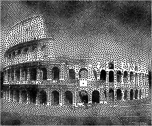
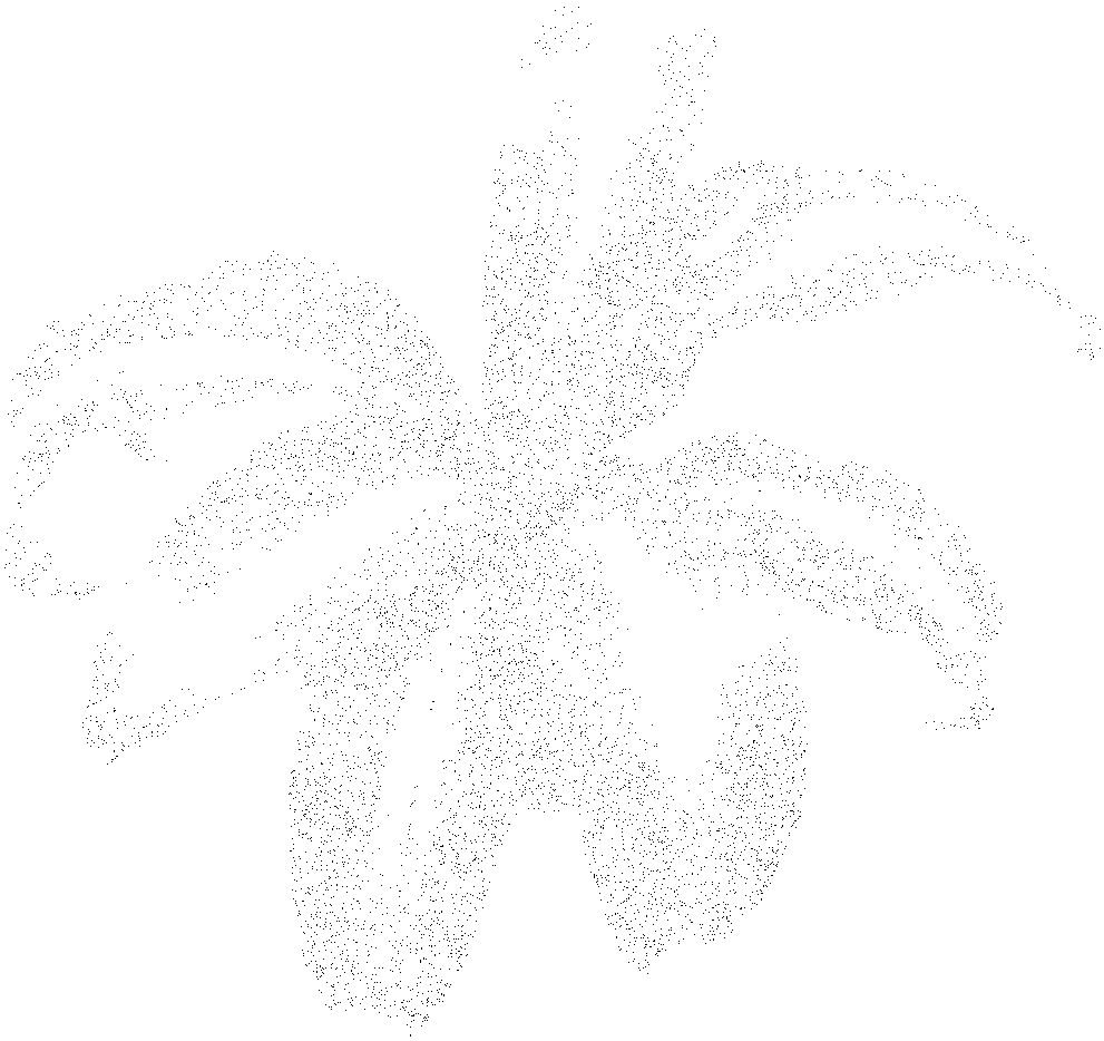
Here is an example of running the algorithm with 12000 stippled with radiuses ranging from 0.3 to 2 after 30 iterations.

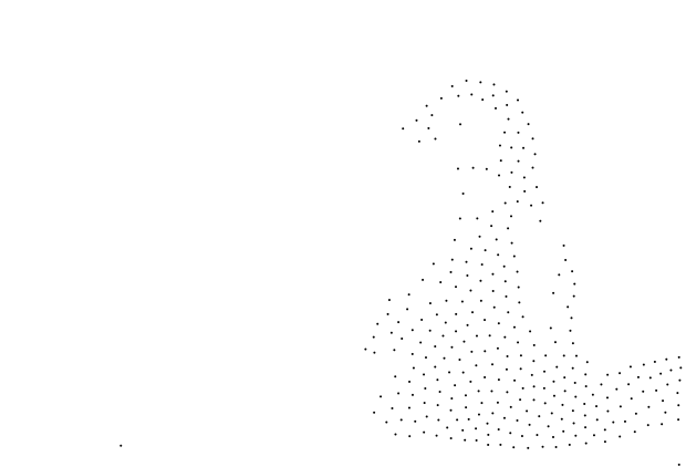
In another fashion here is the penguin in my previous blog post stippled with 300 points of the same size. This doesn’t look like much but the points outline the shape of the penguin quite well. This is a good candidate for reproducing TSP art, which I will be doing in another blog post, but not yet.

Conclusion

It took me quite some time to nail down the details. At first I started manipulating integers and I couldn’t figure out why my results were off. My “breakthrough” was to decompose the computation from the rendering, which with hindsight makes perfect sense. This is the whole idea of vector versus raster graphics. Using points with floating point coordinates for computation reduces rounding errors and allows to compute sub-pixel details.

I realize I went quickly through some of the details, this is simply because I didn’t want to write a two-hour post. If you have questions or suggestions please feel free to contact me. As usual the code is available on GitHub.