Focal loss implementation for LightGBM
Table of contents
Edit (2021-01-26) – I initially wrote this blog post using version 2.3.1 of LightGBM. I’ve now updated it to use version 3.1.1. There are a couple of subtle but important differences between version 2.x.y and 3.x.y. If you’re using version 2.x.y, then I strongly recommend you to upgrade to version 3.x.y.
Motivation
If you’re reading this blog post, then you’re likely to be aware of LightGBM. The latter is a best of breed gradient boosting library. As of 2020, it’s still the go-to machine learning model for tabular data. It’s also ubiquitous in competitive machine learning.
One of LightGBM’s nice features is that you can provide it with a custom loss function. Depending on what you’re doing, this may have a big positive impact. For instance, it was a major part of every top solution to the recent M5 forecasting competition on Kaggle. In this post, I want to do an in-depth presentation of how to implement the loss function described in Focal Loss for Dense Object Detection, which was written by members of the FAIR research group. Focal loss was initially proposed to resolve the imbalance issues that occur when training object detection models. However, it can and has been used for many imbalanced learning problems. Focal loss is just a loss function, and may thus be used in conjunction with any model that uses gradients, including neural networks and gradient boosting. If you implement it as part of a deep learning framework such as PyTorch, then you don’t have to worry too much because the gradient will automatically be computed for you. See here for a PyTorch implementation of focal loss. However, LightGBM doesn’t provide this functionality, thus requiring users to manually implement gradients.
There’s quite a few “guides” on how to implement focal loss for LightGBM. See for instance this somewhat popular GitHub repository as well as this Medium article. Alas, I’m almost certain that each one of them is wrong because some important details are ignored. Trust me, even though they might work on a given dataset, they’re most likely suboptimal. That’s the thing about machine learning code: it might compile and work, but it’s not necessarily correct and optimal. I’ll go over the pitfalls that you’re probably not aware of, and provide some concrete code examples. The goal of this blog post is thus to serve as a comprehensive recipe on how to implement any custom loss function whatsoever in LightGBM. Note that I’ve picked focal loss as a case example because I want to use it for a data science competition.
LightGBM custom loss function caveats
I’m first going to define a custom loss function that reimplements the default loss function that LightGBM uses for binary classification, which is the logistic loss. Doing so will allow me to verify that all the steps I’m taking are correct. Indeed, I will have nothing to compare against when I implement focal loss. If I write a custom implementation of the logarithmic, then I’ll be able to compare it with LightGBM’s implementation. Starting with the logistic loss and building up to the focal loss seems like a more reasonable thing to do. I’ve identified four steps that need to be taken in order to successfully implement a custom loss function for LightGBM:
- Write a custom loss function.
- Write a custom metric because step 1 messes with the predicted outputs.
- Define an initialization value for your training set and your validation set.
- Add the initialization value to the test margins before converting them to probabilities.
Don’t worry if it’s not all clear you, because it certainly was confusing to me when I first started. I’ll go through each step in detail throughout the rest of this notebook. However, first things first: let’s pick a dataset to work with. I’ll be using the credit card frauds dataset. It’s a binary classification dataset with around 30 features, 285k rows, and a highly imbalanced target – it contains much more 0s than 1s. Here is some bash code which you can use to obtain the dataset:
$ curl -O maxhalford.github.io/files/datasets/creditcardfraud.zip
$ unzip creditcardfraud.zip
I’m then going to use the following code to split the data into a training set and a test set. I’m also going to split the training set into a “fitting” set that will be used for training the model, as well as a validation set which will be used for early stopping.
import pandas as pd
from sklearn import model_selection

df = pd.read_csv('creditcard.csv')
X = df.drop(columns='Class')
y = df['Class']

X_train, X_test, y_train, y_test = model_selection.train_test_split(
    X, y,
    random_state=42
)

X_fit, X_val, y_fit, y_val = model_selection.train_test_split(
    X_train, y_train,
    random_state=42
)

X_train.head()
| Time | V1 | V2 | V3 | V4 | V5 | V6 | V7 | V8 | V9 | V10 | V11 | V12 | V13 | V14 | V15 | V16 | V17 | V18 | V19 | V20 | V21 | V22 | V23 | V24 | V25 | V26 | V27 | V28 | Amount |
|---|---|---|---|---|---|---|---|---|---|---|---|---|---|---|---|---|---|---|---|---|---|---|---|---|---|---|---|---|---|
| 59741 | -1.64859 | 1.22813 | 1.37017 | -1.73554 | -0.0294547 | -0.484129 | 0.918645 | -0.43875 | 0.982144 | 1.24163 | 1.10562 | 0.0583674 | -0.659961 | -0.535813 | 0.0472013 | 0.664548 | -1.28096 | 0.184568 | -0.331603 | 0.384201 | -0.218076 | -0.203458 | -0.213015 | 0.0113721 | -0.304481 | 0.632063 | -0.262968 | -0.0998634 | 38.42 |
| 45648 | -0.234775 | -0.493269 | 1.23673 | -2.33879 | -1.17673 | 0.885733 | -1.96098 | -2.36341 | -2.69477 | 0.360215 | 1.6155 | 0.447752 | 0.605692 | 0.169591 | -0.0736552 | -0.163459 | 0.562423 | -0.577032 | -1.63563 | 0.364679 | -1.49536 | -0.0830664 | 0.0746123 | -0.347329 | 0.5419 | -0.433294 | 0.0892932 | 0.212029 | 61.2 |
| 31579 | 1.13463 | -0.77446 | -0.16339 | -0.533358 | -0.604555 | -0.244482 | -0.212682 | 0.0407824 | -1.13663 | 0.792009 | 0.961637 | -0.140033 | -1.25376 | 0.835103 | 0.458756 | -1.3715 | 0.0201648 | 0.796223 | -0.519459 | -0.396476 | -0.684454 | -1.85527 | 0.171997 | -0.387783 | -0.0629846 | 0.245118 | -0.0611777 | 0.0121796 | 110.95 |
| 80455 | 0.0695137 | 1.01775 | 1.03312 | 1.38438 | 0.223233 | -0.310845 | 0.597287 | -0.127658 | -0.701533 | 0.0707389 | -0.857263 | -0.290899 | 0.289337 | 0.333125 | 1.64318 | -0.507737 | -0.0242082 | 0.37196 | 1.56145 | 0.14876 | 0.0970231 | 0.369957 | -0.219266 | -0.124941 | -0.0497488 | -0.112946 | 0.11444 | 0.0661008 | 10 |
| 39302 | -0.199441 | 0.610092 | -0.114437 | 0.256565 | 2.29075 | 4.00848 | -0.12353 | 1.03837 | -0.0758464 | 0.0304526 | -0.75603 | -0.0451648 | -0.18018 | -0.0481675 | -0.00448576 | -0.541172 | -0.17495 | 0.355749 | 1.37528 | 0.292972 | -0.0197334 | 0.165463 | -0.080978 | 1.02066 | -0.30073 | -0.269595 | 0.481769 | 0.254114 | 22 |
As is probably obvious, I’ll be using LightGBM’s Python package. Specifically, I’m running version 2.3.1 3.1.1 with Python 3.7.4 3.8.3. For the time being, I’ll use the generic training API, and not the scikit-learn API. That’s because the former allows more low-level manipulation, whereas the latter is more high-level. Before implementing our custom logistic loss function, let’s run LightGBM so that we have something to compare against:
import lightgbm
from sklearn import metrics

fit = lightgbm.Dataset(X_fit, y_fit)
val = lightgbm.Dataset(X_val, y_val, reference=fit)

model = lightgbm.train(
    params={
        'learning_rate': 0.01,
        'objective': 'binary'
    },
    train_set=fit,
    num_boost_round=10000,
    valid_sets=(fit, val),
    valid_names=('fit', 'val'),
    early_stopping_rounds=20,
    verbose_eval=100
)

y_pred = model.predict(X_test)

print()
print(f"Test's ROC AUC: {metrics.roc_auc_score(y_test, y_pred):.5f}")
print(f"Test's logloss: {metrics.log_loss(y_test, y_pred):.5f}")
Training until validation scores don't improve for 20 rounds
[100]	fit's binary_logloss: 0.0018981	    val's binary_logloss: 0.0035569
[200]	fit's binary_logloss: 0.00080822	val's binary_logloss: 0.00283644
[300]	fit's binary_logloss: 0.000396519	val's binary_logloss: 0.00264941
Early stopping, best iteration is:
[352]	fit's binary_logloss: 0.000281286	val's binary_logloss: 0.00261413

Test's ROC AUC: 0.97772
Test's logloss: 0.00237
Our goal is now to write a custom loss function that will produce the exact same output as above. A custom loss function can be provided the fobj parameter, as specified in the documentation of the train function. Note that “fobj” is short for “objective function”, which is a synonym for “loss function”. As indicated in the documentation, we need to provide a function that takes as inputs (preds, train_data) and returns as outputs (grad, hess). This function will then be used internally by LightGBM, essentially overriding the C++ code that it used by default. Here goes:
from scipy import special

def logloss_objective(preds, train_data):
    y = train_data.get_label()
    p = special.expit(preds)
    grad = p - y
    hess = p * (1 - p)
    return grad, hess
The mathematics that are required in order to derive the gradient and the Hessian are not very involved, but they do require knowledge of the chain rule. I recommend checking out this CrossValidated thread as well as this blog post for more information. One important thing to notice is that the preds array provided by LightGBM contains raw margin scores instead of probabilities. We have thus got to convert them to probabilities ourselves before evaluating the gradient and the Hessian by using a sigmoid transformation. So far, so good. The issue is that the same thing occurs in the metric function. We therefore have to define a custom metric function to accompany our custom objective function. This can be done via the feval parameter, which is short for “evaluation function”. In our case, we can use scikit-learn’s metrics.log_loss function. However, the latter incurs a lot of overhead; it’s much more efficient to implement it ourselves – about 5 times faster in my experience:
import numpy as np

def logloss_metric(preds, train_data):
    y = train_data.get_label()
    p = special.expit(preds)

    ll = np.empty_like(p)
    pos = y == 1
    ll[pos] = np.log(p[pos])
    ll[~pos] = np.log(1 - p[~pos])

    is_higher_better = False
    return 'logloss', -ll.mean(), is_higher_better
All of the guides I’ve read on custom loss functions for LightGBM stop at this point. However, if you set the fobj and feval parameters with the above functions, you’ll see that you don’t obtain the same outputs as when using LightGBM’s implementation. Let me demonstrate:
model = lightgbm.train(
    params={'learning_rate': 0.01},
    train_set=fit,
    num_boost_round=10000,
    valid_sets=(fit, val),
    valid_names=('fit', 'val'),
    early_stopping_rounds=20,
    verbose_eval=100,
    # Notice the two following parameters
    fobj=logloss_objective,
    feval=logloss_metric
)

# Notice how we use a sigmoid here to obtain probabilities
y_pred = special.expit(model.predict(X_test))

print()
print(f"Test's ROC AUC: {metrics.roc_auc_score(y_test, y_pred):.5f}")
print(f"Test's logloss: {metrics.log_loss(y_test, y_pred):.5f}")
Training until validation scores don't improve for 20 rounds
[100]	fit's logloss: 0.203632	    val's logloss: 0.203803
[200]	fit's logloss: 0.0709961	val's logloss: 0.0712959
[300]	fit's logloss: 0.0263333	val's logloss: 0.0267926
[400]	fit's logloss: 0.0103193	val's logloss: 0.0110446
[500]	fit's logloss: 0.00419716	val's logloss: 0.00541233
[600]	fit's logloss: 0.00181725	val's logloss: 0.00341563
[700]	fit's logloss: 0.000777108	val's logloss: 0.00277328
[800]	fit's logloss: 0.000378409	val's logloss: 0.00259164
Early stopping, best iteration is:
[874]	fit's logloss: 0.000237358	val's logloss: 0.00257534

Test's ROC AUC: 0.97701
Test's logloss: 0.00227
As you can see, the test scores are somewhat similar to the previous outputs, but they’re not exactly the same. What’s more, the model has taken around 500 more iterations to converge. When you’re implementing a fancy loss function with nothing to compare against, then it’s virtually impossible to verify that your implementation is correct. In the above case, the scores are close, but that’s not satisfactory.
I didn’t manage myself to find the discrepancy by myself, so I opened a GitHub issue. shiyu1994 kindly made me aware that the problem was that I didn’t specify any initialization values for my model. Indeed, if you look at some gradient boosting algorithm pseudo-code, you’ll see that the model starts off with an initial estimate. From Wikipedia, the latter is defined mathematically as so:
$$\begin{equation} F_0(x) = \mathop{\mathrm{argmin}}\limits_{\zeta} \sum_{i=1}^n L(y_i, \zeta) \end{equation}$$
where
- $y$ is the array of ground truths,
- $n$ is the number of ground truths,
- $L$ is the loss function,
- $\zeta$ is the initialization value we want to find.
Note that I renamed $\gamma$ in the Wikipedia article on gradient boosting to $\zeta$ because I’ll be using $\gamma$ in the focal loss definition later on. Essentially, $\zeta$ is the value used to initialise the gradient boosting algorithm. This is mainly done to speed up convergence. The trick is that the definition of $\zeta$ depends on the loss function. Therefore, we need to provide a value for $\zeta$ if we specify a custom loss function. By default, it seems that LightGBM defaults to $\zeta = 0$, which is sub-optimal. To be honest, I don’t think that a lot of data scientists are aware of this fact, even seasoned Kagglers. It’s not their fault, though. In my opinion, LightGBM should raise a warning when a custom loss function is used without a custom initialization value. But that’s just me.
The optimal initialization value for logistic loss is computed in the BoostFromScore method of the binary_objective.hpp file within the LightGBM repository. You can also find it in the get_init_raw_predictions method of scikit-learn’s BinomialDeviance class. It goes as follows:
$$\begin{equation} \zeta = \log(\frac{\frac{1}{n}\sum_{i=1}^n y_i}{1 - \frac{1}{n}\sum_{i=1}^n y_i}) \end{equation}$$
This should make sense intuitively, as $\frac{1}{n}\sum_{i=1}^n y_i$ is the average of the ground truths, which feels like the most reasonable default value to pick. The above formula is simply the log-odds of $\frac{1}{n}\sum_{i=1}^n y_i$.
When using the generic Python interface of LightGBM, the initialization values can be specified by setting the init_score parameter of each dataset. Once the model is trained and available for making predictions, we also need to add the initialization score to the raw predictions before applying the sigmoid transformation.
def logloss_init_score(y):
    p = y.mean()
    p = np.clip(p, 1e-15, 1 - 1e-15)  # never hurts
    log_odds = np.log(p / (1 - p))
    return log_odds

fit = lightgbm.Dataset(
    X_fit, y_fit,
    init_score=np.full_like(y_fit, logloss_init_score(y_fit), dtype=float)
)

val = lightgbm.Dataset(
    X_val, y_val,
    init_score=np.full_like(y_val, logloss_init_score(y_fit), dtype=float),
    reference=fit
)

model = lightgbm.train(
    params={'learning_rate': 0.01},
    train_set=fit,
    num_boost_round=10000,
    valid_sets=(fit, val),
    valid_names=('fit', 'val'),
    early_stopping_rounds=20,
    verbose_eval=100,
    fobj=logloss_objective,
    feval=logloss_metric
)

# Notice the change here
y_pred = special.expit(logloss_init_score(y_fit) + model.predict(X_test))

print()
print(f"Test's ROC AUC: {metrics.roc_auc_score(y_test, y_pred):.5f}")
print(f"Test's logloss: {metrics.log_loss(y_test, y_pred):.5f}")
Training until validation scores don't improve for 20 rounds
[100]	fit's logloss: 0.00191083	val's logloss: 0.00358371
[200]	fit's logloss: 0.000825181	val's logloss: 0.00286873
[300]	fit's logloss: 0.000403679	val's logloss: 0.00262094
Early stopping, best iteration is:
[355]	fit's logloss: 0.000282887	val's logloss: 0.00257033

Test's ROC AUC: 0.97721
Test's logloss: 0.00233
I know, this is quite finicky, but it works perfectly! Maybe that future versions of LightGBM will make this process easier, but until now we’re stuck with getting our hands dirty. As far as I know, most tutorials ignore the initialization score details because their authors are simply not aware of it.

For practicality, here is the full code that you can copy/paste into a notebook and execute:
Click to see the full code
import lightgbm
import numpy as np
import pandas as pd
from scipy import special
from sklearn import metrics
from sklearn import model_selection

def logloss_init_score(y):
    p = y.mean()
    p = np.clip(p, 1e-15, 1 - 1e-15)
    log_odds = np.log(p / (1 - p))
    return log_odds

def logloss_objective(preds, train_data):
    y = train_data.get_label()
    p = special.expit(preds)
    grad = p - y
    hess = p * (1 - p)
    return grad, hess

def logloss_metric(preds, train_data):
    y = train_data.get_label()
    p = special.expit(preds)
    is_higher_better = False
    return 'logloss', metrics.log_loss(y, p), is_higher_better

df = pd.read_csv('creditcard.csv')
X = df.drop(columns='Class')
y = df['Class']

X_train, X_test, y_train, y_test = model_selection.train_test_split(
    X, y,
    random_state=42
)

X_fit, X_val, y_fit, y_val = model_selection.train_test_split(
    X_train, y_train,
    random_state=42
)

fit = lightgbm.Dataset(
    X_fit, y_fit,
    init_score=np.full_like(y_fit, logloss_init_score(y_fit), dtype=float)
)

val = lightgbm.Dataset(
    X_val, y_val,
    init_score=np.full_like(y_val, logloss_init_score(y_fit), dtype=float),
    reference=fit
)

model = lightgbm.train(
    params={'learning_rate': 0.01},
    train_set=fit,
    num_boost_round=10000,
    valid_sets=(fit, val),
    valid_names=('fit', 'val'),
    early_stopping_rounds=20,
    verbose_eval=100,
    fobj=logloss_objective,
    feval=logloss_metric
)

y_pred = special.expit(logloss_init_score(y_fit) + model.predict(X_test))

print()
print(f"Test's ROC AUC: {metrics.roc_auc_score(y_test, y_pred):.5f}")
print(f"Test's logloss: {metrics.log_loss(y_test, y_pred):.5f}")
Training until validation scores don't improve for 20 rounds
[100]	fit's logloss: 0.00191083	val's logloss: 0.00358371
[200]	fit's logloss: 0.000825181	val's logloss: 0.00286873
[300]	fit's logloss: 0.000403679	val's logloss: 0.00262094
Early stopping, best iteration is:
[355]	fit's logloss: 0.000282887	val's logloss: 0.00257033

Test's ROC AUC: 0.97721
Test's logloss: 0.00233
Now that we know what steps to take, let’s move on to the case of focal loss.
Formulas for focal loss
Let’s start by going over some equations and briefly explain how focal loss works. The mathematical definition of focal loss is given by equation 5 of the paper I mentioned at the beginning of this post:
$$\begin{equation} FL(p_t) = -a_t (1 - p_t)^{\gamma} \log(p_t) \end{equation}$$
The variable $p_t$ is a function of the ground truth $y$ and a prediction $p$:
$$\begin{equation} p_t = \begin{cases} p & \text{if } y = 1 \\ 1 - p & \text{otherwise} \end{cases} \end{equation}$$
Basically, $p_t$ is introduced to simplify notation. Note that $p$ is obtained by applying the sigmoid function to the raw margins $z$:
$$\begin{equation} p = \frac{1}{1 + e^{-z}} \end{equation}$$
In fact, $z$ is denoted by $x$ in the paper’s appendix, but I find that confusing. Additionally, the authors assume that $y \in \{-1, 1\}$ instead of $y \in \{0, 1\}$, which has its importance. Meanwhile, $\alpha_t$ is another parameter with the following definition:
$$\begin{equation} \alpha_t = \begin{cases} \alpha \in [0, 1] & \text{if } y = 1 \\ 1 - \alpha & \text{otherwise} \end{cases} \end{equation}$$
It’s important to understand that $p_t$ and $\alpha_t$ are just artificial variables that are introduced to ease the notation. Indeed, the focal loss can rewritten in terms of $y$ and $p$ instead:
$$\begin{equation} FL(y, p) = -\frac{y + 1}{2} \times \alpha (1 - p)^\gamma \log(p) - \frac{1 - y}{2} \times (1 - a) p^\gamma \log(1 - p) \end{equation}$$
Note that the above equation assumes $y \in \{-1, 1\}$. If on the contrary $y \in \{0, 1\}$, then the following definition applies:
$$\begin{equation} FL(y, p) = -y \times \alpha (1 - p)^\gamma \log(p) - (1 - y) \times (1 - a) p^\gamma \log(1 - p) \end{equation}$$
First order derivative
The authors of the paper provide the derivative of focal loss with respect to the model’s output $z$ in appendix B:
$$\begin{equation} \frac{\partial FL}{\partial z} = \alpha_t y (1 - p_t)^{\gamma} (\gamma p_t \log(p_t) + p_t - 1) \end{equation}$$
Alas, the authors do not provide the second order derivative, so we’ll have to work it out ourselves. But first, in order to warm up, I’ll go through the steps required to obtain the first order derivative. The latter can be obtained by applying the chain rule:
$$\begin{equation} \frac{\partial FL}{\partial z} = \frac{\partial FL}{\partial p_t} \times \frac{\partial p_t}{\partial p} \times \frac{\partial p}{\partial z} \end{equation}$$
The first part of the chain is the most complicated part, as it is the derivative of a product of three elements:
$$\begin{equation} \begin{split} \frac{\partial FL}{\partial p_t} & = \alpha_t \gamma (1 - p_t)^{\gamma - 1} \log(p_t) - \frac{\alpha_t(1 - p_t)^{\gamma}}{p_t} \\ & = \alpha_t(1 - p_t)^{\gamma} (\frac{\gamma \log(p_t)}{1 - p_t} - \frac{1}{p_t}) \\ & = \alpha_t(1 - p_t)^{\gamma} (\frac{\gamma p_t \log(p_t) + p_t - 1)}{p_t(1 - p_t)}) \end{split} \end{equation}$$
The second part of the chain is the derivative of $p_t$ with respect to $p$. The trick is to flatten out $p_t$ into a single formula:
$$\begin{equation} p_t = \frac{p(y + 1)}{2} + \frac{(1 - p)(1 - y)}{2} \end{equation}$$
The derivative then boils down to:
$$\begin{equation} \begin{split} \frac{\partial p_t}{\partial p} & = \frac{y + 1}{2} + \frac{y - 1}{2} \\ & = \frac{2y}{2} \\ & = y \end{split} \end{equation}$$
Finally, the last part of the chain is the well-known gradient of the sigmoid function, thus:
$$\begin{equation} \frac{\partial p}{\partial z} = p(1 - p) \end{equation}$$
As it happens, $p(1 - p)$ is equal to $p_t (1 - p_t)$. Therefore, some terms get cancelled out nicely once the chain parts are multiplied with each other:
$$\begin{equation} \begin{split} \frac{\partial FL}{\partial z} & = \alpha_t(1 - p_t)^{\gamma} (\frac{\gamma p_t \log(p_t) + p_t - 1)}{p_t(1 - p_t)}) \times y \times p_t (1 - p_t) \\ & = \alpha_t y (1 - p_t)^{\gamma} (\gamma p_t \log(p_t) + p_t - 1) \end{split} \end{equation}$$
We know that this derivative is correct because the focal loss authors – who look like stand up guys – provide it in their paper. Additionally, it’s easy to see that setting $a_t = 1$ and $\gamma = 0$ leads to the derivative of cross-entropy – which is also given in the paper. So far, so good.
Second order derivative
Now for the second order derivative, which can be obtained by differentiating the gradient we’ve just obtained with respect to $z$:
$$\begin{equation} \begin{split} \frac{\partial^2 FL}{\partial z^2} & = \frac{\partial}{\partial z} (\frac{\partial FL}{\partial z}) \\ & = \frac{\partial}{\partial p_t} (\frac{\partial FL}{\partial z}) \times \frac{\partial p_t}{\partial p} \times \frac{\partial p}{\partial z} \end{split} \end{equation}$$
We’ve already computed the last two parts of the chain, which are respectfully equal to $y$ and $p(1 - p)$. Therefore, we just have to compute the first part of chain’s first derivative. In order to make things easier, let’s use the following notation:
$$\begin{equation}\frac{\partial FL}{\partial z} = u \times v\end{equation}$$
$$\begin{equation}u = \alpha_t y (1 - p_t)^\gamma\end{equation}$$
$$\begin{equation}v = \gamma p_t \log(p_t) + p_t - 1\end{equation}$$
The derivatives of $u$ of $v$ with respect to $p_t$ are quite straightforward:
$$\begin{equation}\frac{\partial u}{\partial p_t} = -\gamma \alpha_t y (1 - p_t)^{\gamma - 1} \end{equation}$$
$$\begin{equation}\frac{\partial v}{\partial p_t} = \gamma \log(p_t) + \gamma + 1\end{equation}$$
The second order derivative is thus:
$$\begin{equation} \frac{\partial^2 FL}{\partial z^2} = (\frac{\partial u}{\partial p_t} \times v + u \times \frac{\partial v}{\partial p_t}) \times \frac{\partial p_t}{\partial p} \times \frac{\partial p}{\partial z} \end{equation}$$
Initialization constant
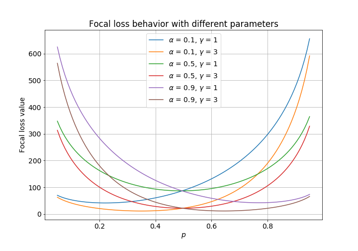
The optimal initialization constant can be derived by differentiating the loss function with respect to $p$. The goal is then to find the value for $p$ which sets the gradient to 0. I gave it a go with pen and paper, but didn’t manage to solve it. I then remembered that most loss functions are convex, and are therefore easy to minimize numerically.
The following plot shows the behavior of focal loss with different sets of parameters. The ground truths are chosen arbitrarily, whilst the initialization value is represented on the $x$-axis. The loss is convex in every case. I therefore gave up on the mathematics and decided to use scipy’s optimize module instead. Numeric optimization is slower than an analytical solution, but I have a hunch that the added cost is trivial.
Implementation
In terms of code, I’m going to organize things a bit differently to the logistic loss case. As we saw in the previous section, there are quite a few functions to implement in order to use a custom loss function. Therefore, I think that it makes sense to organize them into a class. This also makes sense because the focal loss has parameters. By using a class, we only have to declare the parameters once, and can reuse them within each method. This avoids us having to add redundant parameters to the signature of each function.
import numpy as np
from scipy import optimize
from scipy import special

class FocalLoss:

    def __init__(self, gamma, alpha=None):
        self.alpha = alpha
        self.gamma = gamma

    def at(self, y):
        if self.alpha is None:
            return np.ones_like(y)
        return np.where(y, self.alpha, 1 - self.alpha)

    def pt(self, y, p):
        p = np.clip(p, 1e-15, 1 - 1e-15)
        return np.where(y, p, 1 - p)

    def __call__(self, y_true, y_pred):
        at = self.at(y_true)
        pt = self.pt(y_true, y_pred)
        return -at * (1 - pt) ** self.gamma * np.log(pt)

    def grad(self, y_true, y_pred):
        y = 2 * y_true - 1  # {0, 1} -> {-1, 1}
        at = self.at(y_true)
        pt = self.pt(y_true, y_pred)
        g = self.gamma
        return at * y * (1 - pt) ** g * (g * pt * np.log(pt) + pt - 1)

    def hess(self, y_true, y_pred):
        y = 2 * y_true - 1  # {0, 1} -> {-1, 1}
        at = self.at(y_true)
        pt = self.pt(y_true, y_pred)
        g = self.gamma

        u = at * y * (1 - pt) ** g
        du = -at * y * g * (1 - pt) ** (g - 1)
        v = g * pt * np.log(pt) + pt - 1
        dv = g * np.log(pt) + g + 1

        return (du * v + u * dv) * y * (pt * (1 - pt))

    def init_score(self, y_true):
        res = optimize.minimize_scalar(
            lambda p: self(y_true, p).sum(),
            bounds=(0, 1),
            method='bounded'
        )
        p = res.x
        log_odds = np.log(p / (1 - p))
        return log_odds

    def lgb_obj(self, preds, train_data):
        y = train_data.get_label()
        p = special.expit(preds)
        return self.grad(y, p), self.hess(y, p)

    def lgb_eval(self, preds, train_data):
        y = train_data.get_label()
        p = special.expit(preds)
        is_higher_better = False
        return 'focal_loss', self(y, p).mean(), is_higher_better
If you’re in a hurry, then the above code is probably what you’re looking for, and you can simply copy/paste it. Here is an overview:
- The focal loss itself is implemented in the
__call__method. - The
init_scoremethod is responsible for providing the initial values. As you can see, it uses theminimize_scalarfunction fromscipyin order to find the best value ofpwith respect to the provided set of parameters. - Note that if
alphais set toNone, then it is essentially ignored. This allows reproducing the behavior of cross-entropy, which is in a sense a special case of focal loss. - The
lgb_objandlgb_evalmethods can be used with LightGBM. I’ll show how to do this in the Benchmarks section. You could easily implement similar methods for XGBoost and CatBoost.
Numerical checks
The FocalLoss implementation is hopefully correct. I say “hopefully” because I’m human and I make mistakes. Therefore, I’m going to write some numerical checks in order to put my mind at ease. We’re doing analysis, therefore we can use the finite difference method to check that our first and second order gradients are correct. It turns out that scipy has a check_grad method. However, I didn’t manage to make it work with vectors as outputs. I thus wrote my own modest gradient checker:
def check_gradient(func, grad, values, eps=1e-8):
    approx = (func(values + eps) - func(values - eps)) / (2 * eps)
    return np.linalg.norm(approx - grad(values))
As you see, check_gradient simply returns the norm of the difference between the output of grad (which is the gradient function we’re checking) and approx (which is the gradient obtained via the finite difference method).
Let’s now generate some random ground truth values, as well as some random probabilities:
np.random.seed(42)
y_true = np.random.uniform(0, 1, 100) > .5
y_pred = np.random.uniform(0, 1, 100)
We can now check that our gradient implementation is correct:
fl = FocalLoss(alpha=.3, gamma=2)

check_gradient(
    func=lambda x: fl(y_true, x),
    grad=lambda x: fl.grad(y_true, x) / (x * (1 - x)),
    values=y_pred
)
2.3954956968511336e-07
Now you might be wondering why we divide the output of grad. The reason why is because check_gradient varies the values of y_pred. We would thus like to examine the gradient of the loss function with respect to p_t and not z. Therefore, we need to divide our gradient by $\frac{\partial p}{\partial z}$, which is equal to p(1 - p).
Let’s run these checks for different values of $\alpha$ and $\gamma$, and verify that the error is always reasonably low:
for gamma in [0, 1, 2, 3]:
    for alpha in [.1, .3, .5, .7, .9]:
        fl = FocalLoss(alpha=alpha, gamma=gamma)
        diff = check_gradient(
            func=lambda x: fl(y_true, x),
            grad=lambda x: fl.grad(y_true, x) / (x * (1 - x)),
            values=y_pred
        )
        assert diff < 1e-6
We can do the same thing for the second order derivative:
for gamma in [0, 1, 2, 3]:
    for alpha in [.1, .3, .5, .7, .9]:
        fl = FocalLoss(alpha=alpha, gamma=gamma)
        diff = check_gradient(
            func=lambda x: fl.grad(y_true, x),
            grad=lambda x: fl.hess(y_true, x) / (x * (1 - x)),
            values=y_pred
        )
        assert diff < 1e-6
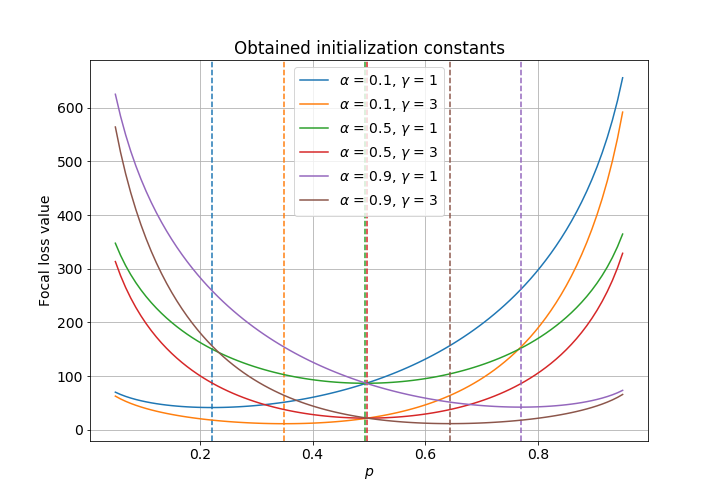
Now, the last thing to check is that the initialization constant is correct. We can check this visually by plotting the value of the average focal loss for different initialization values. If our implementation is correct, then the initialization value should coincide with the minimum value of the focal loss. That seems to be the case on the following figure.
Click to see the code
import matplotlib
import matplotlib.pyplot as plt
from scipy import special

fig, ax = plt.subplots(figsize=(10, 7))
matplotlib.rc('font', size=14)

np.random.seed(10)
y = np.random.randint(2, size=500)  # random 0s and 1s

for alpha in [.1, .5, .9]:
    for gamma in [1, 3]:
        fl = FocalLoss(alpha=alpha, gamma=gamma)
        ps = np.linspace(5e-2, 1 - 5e-2, 100)
        ls = [fl(y, p).sum() for p in ps]

        curve = ax.plot(ps, ls, label=r'$\alpha$ = %s, $\gamma$ = %s' % (alpha, gamma))[0]
        p = special.expit(fl.init_score(y))
        ax.axvline(p, color=curve.get_color(), linestyle='--')

ax.legend()
ax.grid()
ax.set_title('Obtained initialization constants')
ax.set_xlabel(r'$p$')
ax.set_ylabel('Focal loss value')
fig.savefig('focal_loss_min.png')
Note that all of the numeric checks we have just ran depend on the values of y_true and y_pred. If you’re going to use this as part of software that’s going to send people to Mars, then I would recommend being more thorough. Hey, this is just a blog post.
Benchmarks
We’ve implemented focal loss along with its first and second order gradients, as well as the correct initialization value. We’re also reasonably confident that our implementation is correct. Let’s now see how this performs on the credit card frauds dataset. The whole point of this exercise is that, supposedly, focal loss works better than logistic loss on imbalanced datasets.
I played around with alpha and gamma, but didn’t really manage to reach a test set ROC AUC score that was convincingly better than what I obtained with logistic loss – which was 0.97721. A mildly interesting fact is that setting alpha=None and gamma=0 performs slightly better than when using logistic loss. The discrepancy is due to the initialization score. The following snippet shows how to go about using the FocalLoss with LightGBM:
import lightgbm
import numpy as np
import pandas as pd
from scipy import optimize
from scipy import special
from sklearn import metrics
from sklearn import model_selection

df = pd.read_csv('creditcard.csv')
X = df.drop(columns='Class')
y = df['Class']

fl = FocalLoss(alpha=None, gamma=0)

X_train, X_test, y_train, y_test = model_selection.train_test_split(
    X, y,
    random_state=42
)

X_fit, X_val, y_fit, y_val = model_selection.train_test_split(
    X_train, y_train,
    random_state=42
)

fit = lightgbm.Dataset(
    X_fit, y_fit,
    init_score=np.full_like(y_fit, fl.init_score(y_fit), dtype=float)
)

val = lightgbm.Dataset(
    X_val, y_val,
    init_score=np.full_like(y_val, fl.init_score(y_fit), dtype=float),
    reference=fit
)

model = lightgbm.train(
    params={'learning_rate': 0.01},
    train_set=fit,
    num_boost_round=10000,
    valid_sets=(fit, val),
    valid_names=('fit', 'val'),
    early_stopping_rounds=20,
    verbose_eval=100,
    fobj=fl.lgb_obj,
    feval=fl.lgb_eval
)

y_pred = special.expit(fl.init_score(y_fit) + model.predict(X_test))

print()
print(f"Test's ROC AUC: {metrics.roc_auc_score(y_test, y_pred):.5f}")
print(f"Test's logloss: {metrics.log_loss(y_test, y_pred):.5f}")
Training until validation scores don't improve for 20 rounds
[100]	fit's focal_loss: 0.00190475	val's focal_loss: 0.00356043
[200]	fit's focal_loss: 0.000811846	val's focal_loss: 0.00285806
[300]	fit's focal_loss: 0.000401933	val's focal_loss: 0.00267161
Early stopping, best iteration is:
[345]	fit's focal_loss: 0.000297174	val's focal_loss: 0.00263719

Test's ROC AUC: 0.97948
Test's logloss: 0.00237
Conclusion
I haven’t bothered with a more thorough benchmarking session because this blog post is already quite long. However, I am confident that my implementation of focal loss is correct. I will thus be using it the next time a wild imbalanced problem appears in front of me. Hopefully it will help. On a more macro point of view, the thing to remember is that the steps I have detailed above can be applied to other loss functions. Feel free to leave a comment if you have any questions.