What my PhD was about
Table of contents
I defended my PhD thesis on the 12th of October 2020, exactly 3 years and 11 days after having started it. The title of my PhD is Machine learning for query selectivity estimation in relational databases. I thought it would be worthwhile to summarise what I did. Note sure anyone will read this, but at least I’ll be able to remember what I did when I grow old and senile.
TLDR
I contributed to making relational database queries go brrr.
More seriously
Relational databases are ubiquitous in most companies around the world. You might not know it, but there’s always a high change that the app/website you’re using is backed by a relational database. On the one hand, people use them store data. On the other hand, people use them to answer questions by querying the data. The focus of my PhD was on the latter.
In a relational database, data record are stored in tables. For instance, if we were recording item purchases in shops, then we might have something like so:

Typically, relations are normalised. Essentially, this means that the data isn’t stored in a single relation. The data is instead scattered across multiple relations. References are used to associates rows with each other. In the above case, we can split the relation into three so-called “dimension tables” and one “fact table”.

Normalisation has a lot of benefits, one of them being that it avoids redundancies. However, as I will try to make evident throughout this post, analysing data that is scattered across relations is a pain in the neck. Indeed, the tools that statisticians have at their disposal are typically made to process data that belongs to a single relation/entity. Of course, the data from the subrelations, can be joined back together, but this is a costly operation that is avoided at all cost in certain situations.
As I mentioned, the focus of my PhD was on the querying aspect of databases. Users issue queries to the database via an interrogation language, which in 99% of cases is some flavor of SQL. For example, the following query can be used to count the number of meatball purchases that were made by blond Swedes in Ikea stores:
SELECT COUNT(*)

-- Relations
FROM customers, shops, items, purchases

-- Joins
WHERE purchases.customer = customers.id
    AND purchases.shop = shops.id
    AND purchases.item = items.id

-- Filters
AND customers.nationality = 'Swedish'
    AND customers.hair = 'Blond'
    AND items.name = 'Meatballs'
    AND shops.name = 'Ikea'
Note that a lot of users also use ORMs, which translate logic that is written in a given object-oriented programming language into SQL. Also note that by user I’m not just referring to human brings that breath and go to the toilet; indeed a lot of database systems are typically interacted with via other computer systems that are controlled by more human-friendly interfaces. Anyway, what matters is that databases are queried via a declarative language, namely SQL. You tell the database what you want, but not how to retrieve it. The database will handle all the details for you and just spit our the result, which is wonderful when you think about it.
From an outside perspective, databases are simple: you query them and they produce a result. In fact, all the complexity of manipulating the data is delegated to the database. The database’s goal is to take your SQL query and convert it into a sequence of steps that it will in order to answer the query. To be precise, the database is divided into different modules that handle different parts of this process. For instance, the query compiler is in charge of translating the SQL query into a sequence of instructions, whilst the query executor is responsible for running said instructions. Of course, all this has to happen as fast as possible in order to satisfy the user. Satisfation is typically defined via an SLA when the database is managed by a cloud provider.
The query compiler outputs a query execution plan (QEP for short). A QEP is a sequence of operations that have to be executed by the query executor in order to answer the associated SQL query. A QEP is a tree, where each node is an operator (such as a JOIN or a WHERE). Each leaf node represents a relation (such as customers, shops, etc.). The problem is that there a lot of QEPs that can answer a given query. In other words, there are many different ways to organise a sequence of operations in order to answer the same SQL query. The goal, as you might expect, is to find the fastest QEP. Indeed, the running times of the QEPs can (widely) vary. For instance, the three following QEPs all answer the same query, they just arrange the necessary operations in a different order:


What changed between each of the above QEPs is the order in which the relations are joined with each other. This might seem harmless to the uninitiated eye, but in practice it can make the different between making a query run in 1 second or 1 hour. To summarise:
- A user issues an SQL query to a database.
- Each query can be answered with many different query execution plans.
- The query optimiser searches for the fastest execution plan.
- The best plan is executed, the results are returned to the user.
The query optimiser searches for the best QEP by enumerating all the ones that are possible. The query optimiser is full of heuristics that it uses to discard candidates QEPs that it knows have no chance of being the best QEP. For instance, it only considers QEPs that “push-down” the WHERE as low as possible in the QEP. This process is called logical optimisation. It’s a low hanging fruit that is used in every serious query optimiser (for instance see bullet 4 of this piece of documention from Amazon Redshift, as well as the Apache Calcite paper).
Once the query optimiser has enumerated a list of candidate QEPs, it has to pick the one which it thinks will perform best by determining the time they will take. The problem is that executing a QEP is the only way to determine the exact time said QEP will take. Alas, executing a QEP in order to determine its running time defeats the purpose of our endeavour. Indeed, we want to determine the best QEP without having to execute it. The only way to proceed is to guess the running time by analysing the structure of the QEP. This is called cost modeling.
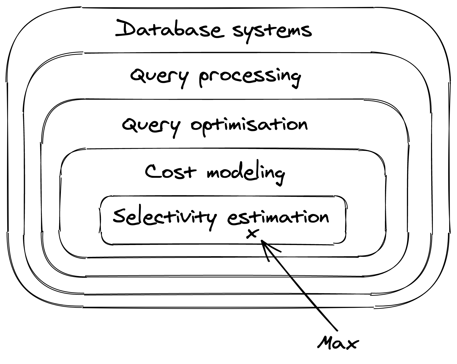
Cost modeling
The query optimiser delegates the task of determining the cost of a QEP to the cost model. In other words, the cost model is a submodule of the query optimisation module, as is shown in the following diagram which represents the lifetime of an SQL query.

The cost model takes as input a QEP and attempts to determine its cost. Note that cost is a loose term. Essentially, its just a number that in an ideal world is strongly correlated with the running time. It doesn’t matter to get it exactly right, what matters is to have a reliable way to rank QEPs according to their cost.
Due to the fact that a QEP is a tree of operators, its cost is the sum of the costs of its operators. An operator refers to an SQL statement, such as a WHERE, a JOIN, or even a GROUP BY. These statements are said to be logical, because they describe what happens to the data. In a QEP, physical operators are instead used. Indeed, a physical operator implements a concrete algorithm that can be executed in order to fulfill the associated logical operator. The textbook example is the JOIN statement, which can be implemented with different algorithms:
- Block nested loop
- Hash join
- Nested loop join
- Sort-merge join
- Symmetric hash join
Each algorithm has its pros and cons. Indeed, one algorithm might be faster than another, but it might also require more live memory. Therefore, in addition to picking the structure of the QEP, a query optimiser also has to decide which physical operators to use! In practice, a run-of-the-mill query with a half-dozen of relations can easily have thousands of candidate QEPs to consider.
Luckily, the cost of an operator can be determined in a straightforward fashion. Indeed, the cost of an algorithm is something that can be derived by looking at what it does and what kind of data structures it uses. For instance, the cost of a nested loop join is proportional to $m \times n$, where $m$ is the length of the left-hand side relation and $n$ is the length of the right-hand side relation. I say proportional because the true cost also has to incorporate the time it takes to process one row, the time it takes to read a page of data from the disk, the time it takes to transfer a chunk of data in case of a network transfer, etc. But these variables don’t have too much impact; what matters most is that the cost is a function of $m$ and $n$.
This is where cost modeling breaks down. Although the formula for determining the cost of an operator is easy to determine, you still have to determine its input sizes. In the previous paragraph, the input sizes are $m$ and $n$. For instance, take a nested loop join between purchases and customers. Let’s say that there $300,000$ purchases and $80,000$ customers. The estimated cost of the nested loop join is thus $300,000 \times 80,000 = 24$ billion. The latter is then some multiplied by some constants that determine how long it takes to process one row. What’s important to understand is that it’s easy to determine the cost of the join because the number of purchases and of customers are known. But what happens if, say, we’re joining blond Swedish customers with meatball purchases?
First of all, we need to determine how many blond Swedes there are. We could do this by scanning the customers relation and count how many time we encounter people who are both blond and Swedish. This is the laziest approach and takes too much time in practice. Instead, we can collect figures that summarise the statistical distribution of the relation’s attributes. More on this later.
Secondly, in our example, we need to determine how many purchases were made for meatballs. This requires joining the items and purchases relations, and then counting how rows have the name field set to 'Meatballs'. Alas, we’re now allowed to perform the join ourselves. Indeed, our goal is to determine the cost of the plan without being able to execute any part of it whatsoever! Hopefully you’re started to get the hint: cost modeling is a hard problem.
The difficult part of cost modeling lies in determining the amount of rows that result from a filtering operation. For instance, we need to have some way of answering the question “how many customers are of Swedish nationality and have blond hair?” without scanning the data on-the-fly. We also need to be able to determine the amount of meatball purchases, even though the meatballs information is part of the items relation, not the purchases relation (damn you normalisation). The devil has many faces, and in this case has a name: selectivity estimation. It’s essentially what I’ve been banging my head against for the past three years.
Selectivity estimation
Selectivity estimation is the most important part of cost modeling. If you produce a correct selectivity, then your cost model will produce a correct cost, which in turn allows the query optimiser the pick the plan with the lowest cost. If the selectivity estimate is incorrect, then getting a correct cost estimated is doomed to failure, and picking the best plan boils down to luck.
A lot of ink has been spilled over selectivity estimation. It all started with a seminal paper written by Patricia Selinger published in 1979: Access path selection in a relational database management system. The latter gives a formal description of what I’ve rambling on about until now. The paper proposes a simple way to perform selectivity estimation: histograms. The idea being to precompute histograms for each attribute in the database. In the case of discrete attributes, histograms are just counters. In order to determine how many blond Swedish customers there are, one simply has to look at the counters for hair and nationality.
Wait, what about correlations? The problem of having one histogram per attribute is that you don’t take into account dependencies between attributes. Indeed, if your hair histogram tells you that there are 20% of blond people, and your nationality histogram tells you that there are 30% of Swedish people, how many blond Swedes do you think there are? In her paper, Patricia Selinger proposes to simply multiply both percentages: $0.2 \times 0.3 = 0.06$. In other words, she proposes to assume independency. This is formally known as the “attribute value independence” assumption, or AVI for short. As you might know, Swedish people tend to be blond. Therefore, assuming independence is wrong. As it might turn out, all the Swedish people in our database might be blond! In that case, the percentage of blond Swedes is equal to the percentage of Swedes, which is 30%, and is well above the 6% estimate.
How might we solve this? We could potentially build a two-dimensional histogram over the hair and nationality attributes. Sure, why not. But what if you have hundreds of attributes? The problem is that a histogram over $d$ dimensions takes an amount of space that grows exponentially with $d$. Anything over three dimensions becomes too cumbersome. If, say, you have $25$ dimensions, then you have to build ${25 \choose 3} = 2300$ histograms. We could limit the histograms to attribute we known are dependent with each other, but that’s difficult in itself. In the previous example, we have some prior assumption about the dependency of nationality on hair. In general, we would like to have some generic method that applies to dependencies that aren’t necessarily grounded in human knowledge.
Virtually all database systems have gone down the road of assuming total independence. In practice, making the AVI assumption means that you only have to build $d$ one-dimensional histograms, which is much less cumbersome. The historical tendency has been to ignore dependencies and instead focus on building a lightweight cost model. As it turns out, query optimisers still get things right most of the time. In fact, producing the correct selectivity estimation only matters in a very small number of cases. However, in those cases, getting the selectivity estimation right can make the difference between the query optimiser picking a slugish or a blazing fast QEP. In other words, the query optimiser might make a mistake once in a while, but that mistake might mean that the database is allocated of its resources to processing a long-running QEP, which will its overall performance. Cost modeling, and in particular selectivity estimation, is still not a solved problem. For instance, see this PostgreSQL mailing list thread. As of 2020, a relatively high amount of research is still being poured into it.
Selectivity estimation ≈ density estimation
As you might have picked up by now, selectivity estimation looks uncannily like density estimation. Density estimation is a sub-field of statistics that deals with answering probabilistic queries, such as:
- How many customers?
- How many Swedish customers?
- How many purchases from Ikea?
- How many purchases from Ikea for meatballs?
- How many Swedish customers who bought meatballs from Ikea?
The goal of density estimation is to produce a data structure that can answer all of the above queries in a timely and memory-efficient fashion. For instance, histograms can be seen as one of the simplest ways to perform density estimation. They have a low memory footprint, but they’re not very accurate because they ignore dependencies between attributes.
A lot of density estimation have been proposed for the purpose of selectivity estimation over the years. A lot of histograms have been proposed, both for the one-dimensional cases (see this, this, and this) as well as multi-dimensional cases (see this and this). There have also been some more esoteric proposals, such as this one which uses copulas.
In recent years, due to the regain in interest in machine learning, a lot of sophisticated answers to the selectivity estimation problem have been proposed. These encompass classical machine learning (see this and this), as well as deep learning (see this, this, and this which are all papers that were published in last 2 years). All of these proposals have a lot of good ideas, but in my opinion they won’t see the light of day in practice. The cold truth is that database systems, and in particular query optimisers, require extremely efficient methods. Machine learning is cute, but I don’t see PostgreSQL suddenly switching its cost model when it’s been using plain and simple histograms since its inception. This is especially true for deep learning, which as we all know isn’t exactly grounded in efficiency.
In other words, the industry imposes a hard limit on what we’re allowed to do. I’ve tried to summarise this in the following chart. Ideally, we want to be at the bottom-right. The problem is that we don’t know about any selectivity estimation which makes the cut in terms of performance and can capture dependencies between multiple attributes across relations. Therefore, we have to make do with histograms, which are simple enough to be used in a high-performance cost model.

This performance aspect is something that I’ve always tried to keep in mind during my PhD. I spent the first 4 months powering through research papers in order to get a grasp of what had been proposed in the past. Surprisingly, I didn’t find any of these methods being used in any existing database cost models. It didn’t just seem to be because database systems are too old and haven’t had the time to update themselves. Indeed, even new query optimisers such as that of Facebook’s Presto and Apache Calcite seem to be using histograms to estimate selectivities. To be quite frank, I believe that there’s a disconnect between industry performance requirements and what researchers explore. Deep learning is trending, but what’s point in researching it if it can’t be used anyway? The North Star goal of my PhD was to keep things simple and usable in practice. I settled on using Bayesian networks because it felt to me that they were capable of ticking all the boxes.
Conditional independence to the rescue
Let me recap with some light statistical notions to understand where Bayesian networks bring value:
- A relation is made of $p$ attributes ${X_1, \dots, X_p}$.
- Each attribute $X_i$ follows an unknown distribution $P(X_i)$.
- $P(X_i = x)$ gives us the probability of a predicate (e.g.
name = 'Ikea'). - $P(X_i)$ can be estimated, for example with a histogram.
- The distribution $P(X_i, X_j)$ captures interactions between $X_i$ and $X_j$ (e.g.
name = 'Ikea' AND nationality = 'Swedish'. - Memorising $P(X_1, \dots, X_p)$ takes $\prod_0^p |X_i|$ units of space.
The common practice in cost models is to assume independence between attributes. Let’s assume ${X_1, \dots, X_p}$ are independent with each other:
- We thus have $P(X_1, \dots, X_p) = \prod_0^p P(X_i)$
- Memorising $P(X_1, \dots, X_p)$ now takes $\sum_0^p |X_i|$ units of space
We’ve compromised between accuracy and space. This is the attribute value independence} (AVI) assumption. On the one hand, we can assume a full dependence situation and store big histograms, on the other hand we can assume total independence and store lightweight histograms. As it turns out, we can strike somewhere in the middle by using conditional independence. The latter is based on Bayes’ theorem:
$$P(A, B) = P(B \mid A) \times P(A)$$
For instance:
$$P(hair, country) = P(hair \mid country) \times P(country)$$
In other words, we can say that hair color is conditioned on the nationality attribute. In case of three variables $A$, $B$, and $C$, $A$ are $B$ are conditionally independent if $C$ determines both of them. In which case:
$$P(A, B, C) = P(A \mid C) \times P(B \mid C) \times P(C)$$
Conditional independence can save space without compromising on accuracy. Indeed, we don’t need $P(A, B, C)$ because it contains too much information. We can instead make use of the fact that we know which attributes are independent on each other and store smaller conditional distributions. Of course, this isn’t obvious if you’re not accustomed with this kind of stuff. As my advisors use to tell me: “montre nous un exemple”. Let’s say you have the following relation:
| nationality | hair | salary |
|---|---|---|
| Swedish | Blond | 42000 |
| Swedish | Blond | 38000 |
| Swedish | Blond | 43000 |
| Swedish | Brown | 37000 |
| American | Brown | 35000 |
| American | Brown | 32000 |
Let’s saying that we’re looking build to a statistical summary of the attributes. We might want to use this statistical summary to look for the number of blond Swedes. The truth is:
$$P(\textcolor{royalblue}{Swedish}, \textcolor{goldenrod}{Blond}) = \frac{3}{6} = 0.5$$
By assuming total independence, we get:
$$P(\textcolor{royalblue}{Swedish}) = \frac{4}{6}$$ $$P(\textcolor{goldenrod}{Blond}) = \frac{3}{6}$$ $$P(\textcolor{royalblue}{Swedish}, \textcolor{goldenrod}{Blond}) = P(\textcolor{royalblue}{Swedish}) \times P(\textcolor{goldenrod}{Blond}) = 0.333$$
With conditional independence, we get:
$$P(\textcolor{goldenrod}{Blond} \mid \textcolor{royalblue}{Swedish}) = \frac{3}{4}$$
$$P(\textcolor{royalblue}{Swedish}, \textcolor{goldenrod}{Blond}) = P(\textcolor{goldenrod}{Blond} \mid \textcolor{royalblue}{Swedish}) \times P(\textcolor{royalblue}{Swedish}) = 0.5$$
Pretty cool, right? The $48,000 question is how do we make use of this for selectivity estimation? The answer is Bayesian networks.
Bayesian networks
A Bayesian network is a method for organising conditional independences. A Bayesian network is a special kind of graphical model that can be used for different purposes. Mainly though, Bayesian networks can be used to make sense of a tabular dataset by arranging conditional independences in a topological fashion.

For example, the attributes from the previous relation can be arranged as so:
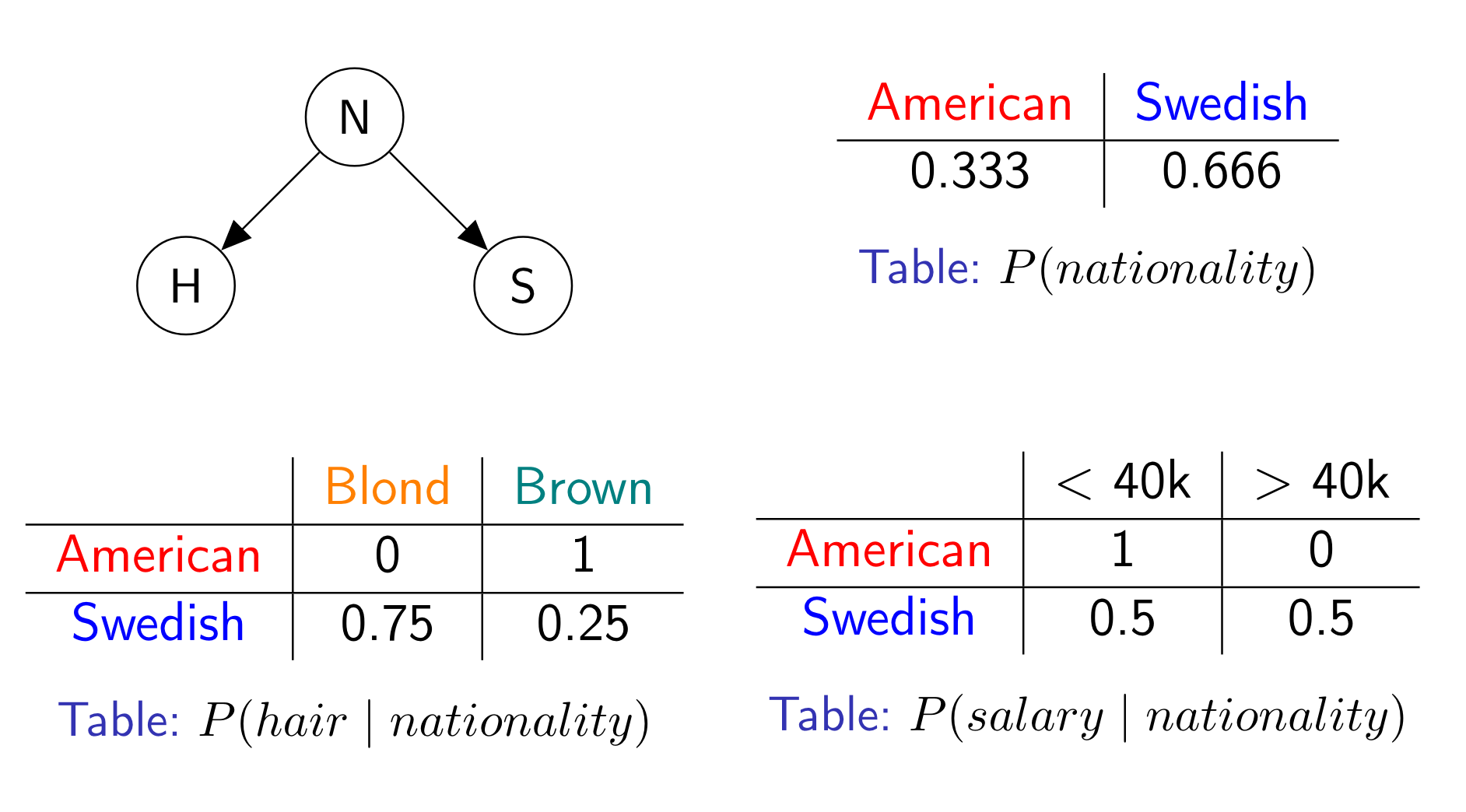
Each node corresponds to an attribute. Each edge indicates a conditional dependency. Each node is associated with a conditional probability distribution (CPD for short). In the above diagram, each CPD is a table because the attributes are discrete (the salary attribute got binned). The Bayesian network as a whole encodes the full joint distribution as so:
$$P(N, H, S) = P(N) \times P(H \mid N) \times P(S \mid N)$$
The Bayesian network can then be queried to answer probabilistic questions, such as the amount of blond Swedes who have a salary above 40k. To do so, the full joint distribution could be reconstructed by multiplying the conditional distributions with each other. That could work, but it would blow up the memory usage. Instead, inference algorithms that traverse the network one node at a time can be used. This is why Bayesian networks are useful: they compress the full joint distribution in a space-efficient manner.
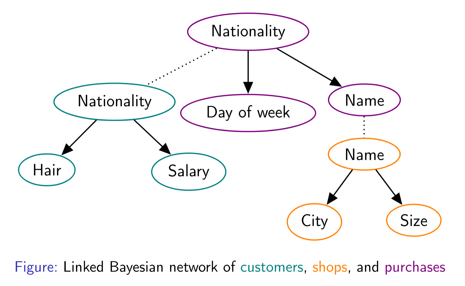
The running time of an inference algorithm depends on the Bayesian network’s structure. The structure also determines the quality of the factorisation. Finding the right structure is of the utmost importance if one is to use Bayesian networks for selectivity estimation. In my work, I focused on Chow-Liu trees. This allowed me to use inference algorithms that run in linear time with respect to the number of attributes. The major contribution of my PhD was to propose a method to build Chow-Liu trees that cover multiple relations.
I don’t want to go into any more detail because I would only be repeating what I’ve written in my research papers. I made a big effort to write these in a clear manner that isn’t overloaded with formulas and abstractions. The two papers I wrote on Bayesian networks for selectivity estimation are:
- An Approach Based on Bayesian Networks for Query Selectivity Estimation
- Selectivity Estimation with Attribute Value Dependencies Using Linked Bayesian Networks
The takeaway from my research is that Bayesian networks seem to be a viable method to improve the histograms used in query optimiser cost models that are used nowadays. Their accuracy is not as high as more sophisticated methods, including deep learning. However, they offer a better tradeoff with respect to performance, and therefore are a more likely candidate.
Conclusion
All in all my PhD was a worthwhile experience. Of course, there were ups and downs. I wasn’t 100% happy with the research environment I was in, but that’s another story. The PhD gave me the time to hone my skills and become a more knowledgeable data scientist. I’m not at all convinced that my work will be used in an industrial grade query optimiser, but I’m certain that I pursued the right research direction. Now I’m working at Alan, with the intent of developing more business acumen, which in my opinion is a key aspect of becoming a great data scientist.
If I had to pick one highlight during my PhD, it would be that I got to go to Thailand for a conference!