Subsampling a training set to match a test set

Edit – it’s 2022 and I still haven’t written a part 2. That’s because I believe this problem is easily solved with adversarial validation.

Some friends and I recently qualified for the final of the 2017 edition of the Data Science Game competition. The first part was a Kaggle competition with data provided by Deezer. The problem was a binary classification task where one had to predict if a user was going to listen to a song that was proposed to him. Like many teams we extracted clever features and trained an XGBoost classifier, classic. However, the one special thing we did was to subsample our training set so that it was more representative of the test set.

One of the basic requirements for a machine learning model to do well is that the data it is trained on and the one it predicts should originate from the same distribution. For example there isn’t much sense in training a model on users who are in their 20s when the users in the test set who are in their 60s. Of course this is never really case, however the previous statement is also somewhat true if users in the test set are in their 30s. Machine learning models learn data representations, or in other words distributions. For each feature, having a distribution in the training set that matches the one in the test set helps a lot.

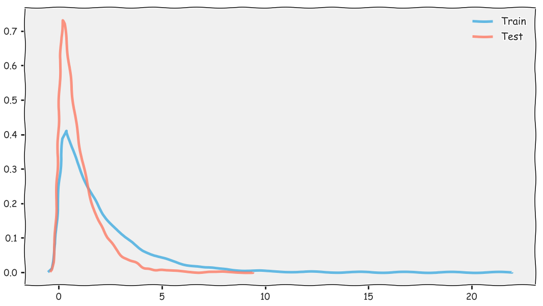
A shift in the test set distribution can occur for many reasons. For example when Facebook split it’s messaging system to a new app called Messenger the average time people spent on the main app probably decreased by a lot, but it probably also didn’t impact churn, quite the contrary I imagine. Shifts like these can occur through time and make part of historical data useless after a while. In the case of the Deezer competition, we had a feature which measured the number of songs a user had listened to up to when the listen occurred. This feature was on average lower than in the training set. In both datasets the data followed an exponential distribution but it was more accentuated in the test set. After subsampling the training set so that this particular feature had the same distribution as in the test set we gained a few percentage points in ROC AUC and climbed the ladder by around 20 spots.

Here is an example of what the difference in distribution looks like. Here and in the rest of the blog I’ll use KDEs to represent distributions.

import matplotlib.pyplot as plt
import numpy as np
import seaborn as sns

plt.style.use('fivethirtyeight')

np.random.seed(0)
train = np.random.exponential(2, size=100000)
test = np.random.exponential(1, size=10000)

with plt.xkcd():
    fig, ax = plt.subplots(figsize=(16, 10))
    sns.kdeplot(train, ax=ax, label='Train', lw=5, alpha=0.6);
    sns.kdeplot(test, ax=ax, label='Test', lw=5, alpha=0.6);
    ax.tick_params(axis='both', which='major', labelsize=18)
    ax.legend(fontsize=20);

expo-example

We want to subsample, say 50000, observations in our training set with the requirement that the subsample’s distribution will match the test set’s one. To do so we have to weight each observation in the training set to express how much it will contribute to matching the test set’s distribution. Intuitively values that are common in the test set but are rare in the training should have a higher weight.

The algorithm that follows should be quite straightforward and is quite fast.

Compute $n$ equal frequency bins from the test
Assign each observation in the training set to the matching bin
For each training set bin $b_i$, count it’s size
Assign weight $\frac{1}{size(b_i)}$ to each observation in the training set belonging to bin $b_i$
Sample $k$ observations from the training set with the weights assigned

The algorithm has two parameters which are the number of bins ($n$) and the size of the subsample ($k$). To generate the equal width bins we can use percentiles.

Now to the code, in Python of course!

SAMPLE_SIZE = 50000
N_BINS = 300

# Obtain `N_BINS` equal frequency bins, in other words percentiles
step = 100 / N_BINS
test_percentiles = [
    np.percentile(test, q, axis=0)
    for q in np.arange(start=step, stop=100, step=step)
]

# Match each observation in the training set to a bin
train_bins = np.digitize(train, test_percentiles)

# Count the number of values in each training set bin
train_bin_counts = np.bincount(train_bins)

# Weight each observation in the training set based on which bin it is in
weights = 1 / np.array([train_bin_counts[x] for x in train_bins])

# Make the weights sum up to 1
weights_norm = weights / np.sum(weights)

np.random.seed(0)
sample = np.random.choice(train, size=SAMPLE_SIZE, p=weights_norm, replace=False)

with plt.xkcd():
    fig, ax = plt.subplots(figsize=(14, 8))
    sns.kdeplot(train, ax=ax, label='Train', lw=5, alpha=0.6);
    sns.kdeplot(test, ax=ax, label='Test', lw=5, alpha=0.6);
    sns.kdeplot(sample, ax=ax, label='Train resampled', lw=5, ls='--', color='gray', alpha=0.6);
    ax.tick_params(axis='both', which='major', labelsize=18)
    ax.legend(fontsize=20);

expo-resample

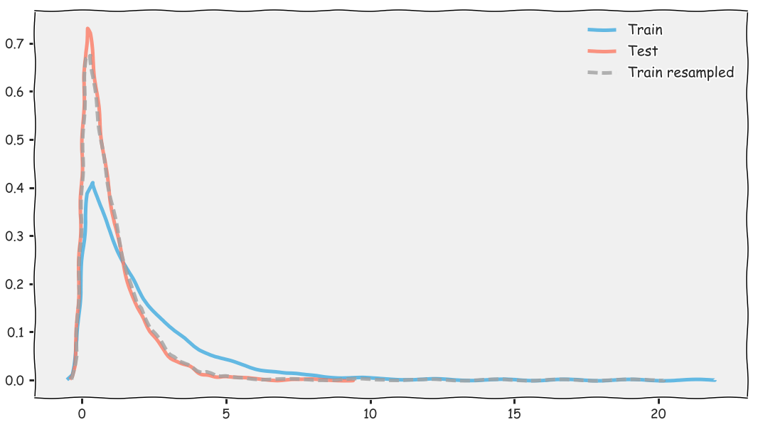
You can see that the subsample (the dashed line) has a similar distribution to the test set (the red). This is exactly what we during the competition. Our initial dataset had around 3 million rows and we actually used a subsample of 1.3 million rows. Less data but more representative data! The number of bins that you use doesn’t matter too much in my experience, and the lower that number the faster the algorithm runs. As for the size of the subsample, the less your training set and test set distributions are difference, the less you will be able to subsample - at least if you are doing it without replacement, which is the only way that makes sense if you don’t want to have duplicates.

I added the subsampling algorithm to my data science package called xam. The next step will be to generalize the weighting and subsampling to multiple dimensions, but that’s for part 2 because I haven’t figured it out yet!

Related posts